Building a GraphSpace
Sysbiolab Team
2026-07-20
Source:vignettes/articles/building-graphspace.Rmd
building-graphspace.Rmd
Package: RGraphSpace 1.4.4
# Check required version
if (packageVersion("RGraphSpace") < "1.4.3"){
  message("Need to update 'RGraphSpace' for this vignette")
  remotes::install_github("sysbiolab/RGraphSpace")
}
Quick start
#--- Load required packages
library("RGraphSpace")
library("igraph")
library("ggplot2")
library("tidygraph")
This section creates a toy igraph from scratch to
demonstrate the vertex and edge attributes that RGraphSpace
parses automatically, showing exactly what the package expects as input.
The same graph can also be supplied as a tidygraph object. Here
we use igraph’s make_star() function and then
V() and E() to assign attributes.
# Make a 'toy' igraph with 5 nodes and 4 edges;
# ..either a directed or undirected graph
gtoy1 <- make_star(5, mode = "out")

# Check whether the graph is directed or not
is_directed(gtoy1)
#> [1] TRUE

# Check graph size
vcount(gtoy1)
#> [1] 5

ecount(gtoy1)
#> [1] 4

# Assign 'x' and 'y' coordinates to each vertex;
# ..this can be an arbitrary unit in (-Inf, +Inf)
V(gtoy1)$x <- c(0, 2, -2, -4, -8)
V(gtoy1)$y <- c(0, 0,  2, -4,  0)

# Assign a name to each vertex
V(gtoy1)$name <- paste0("n", 1:5)
# The most direct call: pass an igraph to plotGraphSpace()
plotGraphSpace(gtoy1, node.labels = TRUE)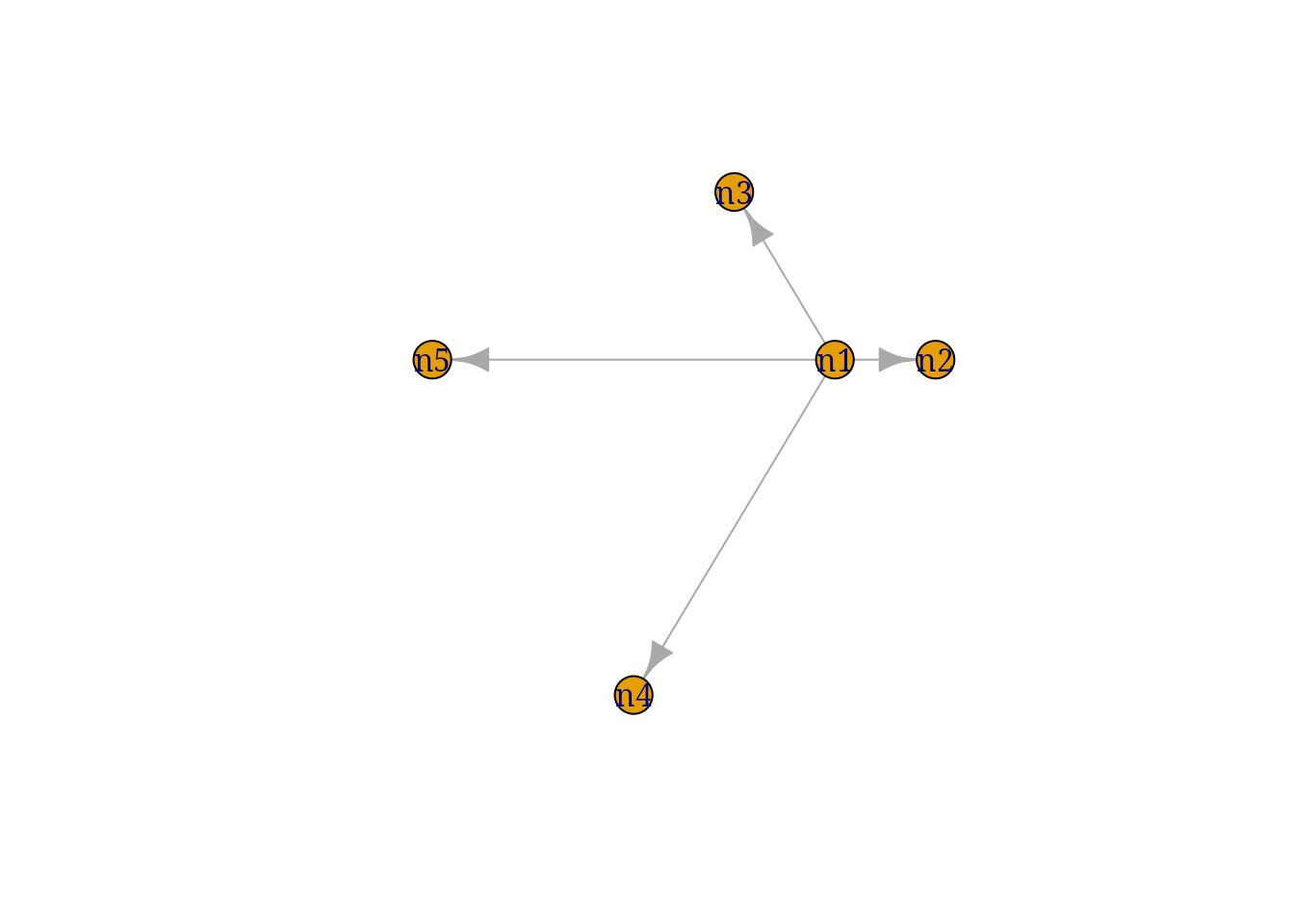
The same graph can be supplied as a tidygraph object; every RGraphSpace entry point accepts it through the same interface.
# Same toy graph, as tidygraph
gr <- as_tbl_graph(gtoy1)
gr
#> # A tbl_graph: 5 nodes and 4 edges
#> #
#> # A rooted tree
#> #
#> # Node Data: 5 × 3 (active)
#>       x     y name
#>   <dbl> <dbl> <chr>
#> 1     0     0 n1
#> 2     2     0 n2
#> 3    -2     2 n3
#> 4    -4    -4 n4
#> 5    -8     0 n5
#> #
#> # Edge Data: 4 × 2
#>    from    to
#>   <int> <int>
#> 1     1     2
#> 2     1     3
#> 3     1     4
#> # ℹ 1 more row
plotGraphSpace(gr, node.labels = TRUE)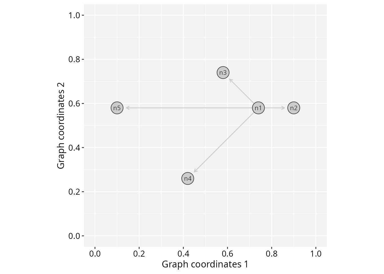
RGraphSpace attributes
Next, we list all vertex and edge attributes that can be passed to RGraphSpace methods.
Vertex attributes
# Node color (Hexadecimal or color name)
V(gtoy1)$nodeColor <- c("red", "#00ad39", "grey80", "lightblue", "cyan")

# Node transparency (in [0,1])
V(gtoy1)$nodeAlpha <- 1

# Node size (numeric in [0, 100], as '%' of the plot space)
V(gtoy1)$nodeSize <- c(8, 5, 5, 10, 5)

# Node shape (integer code between 0 and 25; see 'help(points)')
V(gtoy1)$nodeShape <- c(21, 22, 23, 24, 25)

# Node line width (as in 'lwd' standard graphics; see 'help(gpar)')
V(gtoy1)$nodeLineWidth <- 1

# Node line color (Hexadecimal or color name)
V(gtoy1)$nodeLineColor <- "grey20"

# Node labels ('NA' will omit the label)
V(gtoy1)$nodeLabel <- c("V1", "V2", "V3", "V4", NA)

# Node label size (in mm)
V(gtoy1)$nodeLabelSize <- 3

# Node label color (Hexadecimal or color name)
V(gtoy1)$nodeLabelColor <- "black"
Edge attributes
Given a list of edges, RGraphSpace represents only one edge for each pair of connected vertices. If there are multiple edges connecting the same node pair, it will display the attributes of the first occurrence in the data.
# Edge color (Hexadecimal or color name)
E(gtoy1)$edgeColor <- c("red","green","blue","black")

# Edge transparency (in [0,1])
E(gtoy1)$edgeAlpha <- 1

# Edge line width (as in 'lwd' standard graphics; see 'help(gpar)')
E(gtoy1)$edgeLineWidth <- 0.8

# Edge line type (as in 'lty' standard graphics; see 'help(gpar)')
E(gtoy1)$edgeLineType <- c("solid", "11", "dashed", "2124")
Note: edgeLineColor is deprecated as of version 1.4.3
and replaced by edgeColor.
Arrowhead attributes
Arrowhead in directed graphs: By default, an arrow
will be drawn for each edge according to its left-to-right orientation
in the edge list (e.g. A -> B). If there are
mutual connections, the package will recode the mutual edges to
represent a bidirectional flow.
# Arrowhead types in directed graphs
## Integer or character code:
## 0 = "---", 1 = "-->", -1 = "--|"
E(gtoy1)$arrowType <- 1
Arrowhead in undirected graphs: By default, no arrow will be drawn for undirected graphs. However, arrowheads may be assigned according to the coding below.
# Arrowhead types in undirected graphs
## Integer or character code:
##  0 = "---"
##  1 = "-->",  2 = "<--",  3 = "<->",  4 = "|->"
## -1 = "--|", -2 = "|--", -3 = "|-|", -4 = "<-|"
gtoy1_undir <- igraph::as_undirected(gtoy1, edge.attr.comb = "first")
E(gtoy1_undir)$arrowType <- 1
# Note: in undirected graphs, this attribute overrides
# the edge's orientation in the edge list and adds arrowheads
# to edges that would otherwise be drawn without any
… and plot the fully attributed gtoy1 object.
# Plot the fully attributed 'gtoy1'
plotGraphSpace(gtoy1, node.labels = TRUE)
Passing graphs to geoms
Alternatively, an igraph can be converted to a
GraphSpace object and passed directly to ggplot2
geoms. This gives full access to the ggplot2 layer system for
combining graph elements with other plot types.
# Load the toy graph used in the previous example
data("gtoy1", package = "RGraphSpace")

# Create a GraphSpace object
gs <- GraphSpace(gtoy1)
#> Validating the 'igraph' object...
#> Ignoring graph-level attributes: 'name', 'mode', 'center'
#> Creating a 'GraphSpace' object...

# Normalize the coordinates
gs <- normalizeGraphSpace(gs)
#> Normalizing node coordinates to graph space...

gs
#> A GraphSpace-class object for:
#> IGRAPH 5fb8aab DN-- 5 4 --
#> + attr: x (v/n), y (v/n), name (v/c), nodeLabel (v/c), nodeLabelSize
#> | (v/n), nodeLabelColor (v/c), nodeShape (v/n), nodeSize (v/n),
#> | nodeColor (v/c), nodeLineWidth (v/n), nodeLineColor (v/c), nodeAlpha
#> | (v/n), edgeLineType (e/c), edgeColor (e/c), edgeLineWidth (e/n),
#> | arrowType (e/n), edgeAlpha (e/n)
#> + node spatial boundaries: normalized to graph space
#> | x: [-8, 2] -> [0, 1] (cols)
#> | y: [-4, 2] -> [0, 1] (rows)
normalizeGraphSpace() maps all vertex coordinates to a
[0, 1] unit interval and computes the per-node clipping
offsets that allow geom_edgespace() to terminate edges
precisely at node boundaries. This step is handled automatically when
you use plotGraphSpace(), but must be called explicitly
when building a plot layer by layer.
# Build a layered ggplot2 graph
# geom_edgespace() draws edges; geom_nodespace() draws nodes
# aes(label = nodeLabel) maps the 'nodeLabel' vertex attribute to node labels
ggplot(gs) +
  geom_edgespace() +
  geom_nodespace(aes(label = nodeLabel), label_size = 3) +
  theme_gspace_coords(is_norm = TRUE)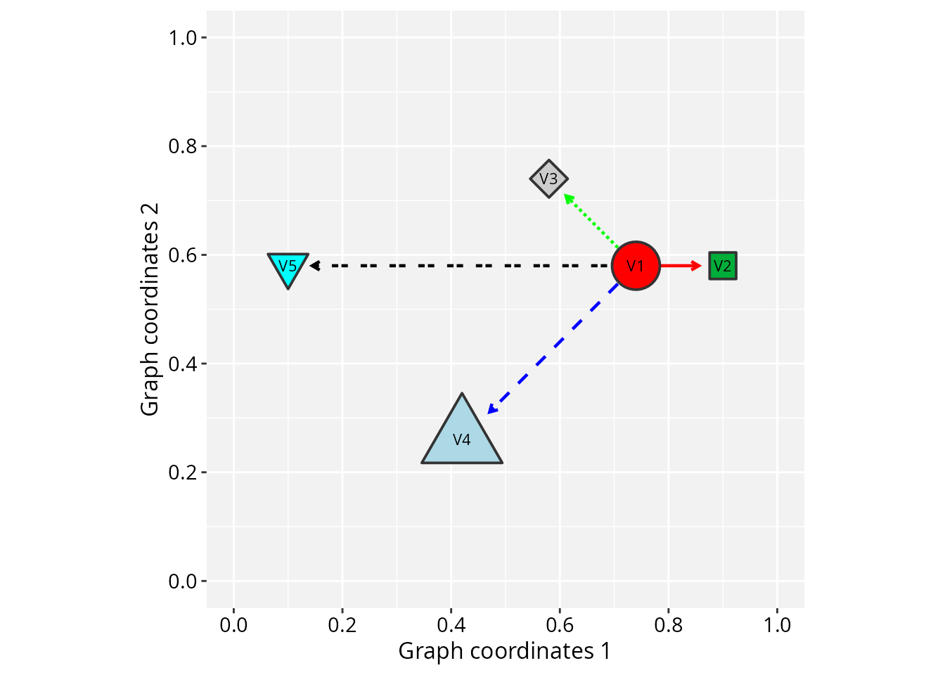
For detailed integration with the ggplot2 ecosystem and other spatial packages, see customizing aesthetics and interoperability with ggraph & sf vignettes.
Choosing an entry point
RGraphSpace provides three levels of access, each suited to a different workflow.
Level 1 — Direct plot from an igraph:
The simplest call requires no intermediate objects. Use this for quick
inspection or when no ggplot2 customization is needed.
# The simplest call
plotGraphSpace(gtoy1, node.labels = TRUE)
Level 2 — Layered plot via
geom_graphspace(): Convert the igraph
to a GraphSpace object first, then pass it to
ggplot2. geom_graphspace() adds node and edge
layers in a single call and gives full access to ggplot2
themes, scales, and annotations.
# Adds node and edge layers in a single call
gs <- GraphSpace(gtoy1)
ggplot(gs) +
  geom_graphspace(aes(label = nodeLabel))
Level 3 — Independent node and edge layers: Use
geom_nodespace() and geom_edgespace() directly
when node and edge layers require separate aesthetic mappings or
independent scale control.
# Set some variables
V(gtoy1)$node_var <- runif(vcount(gtoy1))
E(gtoy1)$edge_var <- runif(ecount(gtoy1))

# Independent node and edge layers
gs <- GraphSpace(gtoy1)
ggplot(gs) +
  geom_edgespace(aes(colour = edge_var)) +
  geom_nodespace(aes(fill = node_var))
The layout argument of GraphSpace() can be
used at levels 2 and 3 to supply coordinates from any igraph
layout algorithm when the graph has no pre-existing x and
y vertex attributes:
# Entry point layout
gs <- GraphSpace(gtoy1, layout = igraph::layout_with_fr(gtoy1))
Session information
#> R version 4.6.1 (2026-06-24)
#> Platform: x86_64-pc-linux-gnu
#> Running under: Ubuntu 24.04.4 LTS
#>
#> Matrix products: default
#> BLAS:   /usr/lib/x86_64-linux-gnu/openblas-pthread/libblas.so.3
#> LAPACK: /usr/lib/x86_64-linux-gnu/openblas-pthread/libopenblasp-r0.3.26.so;  LAPACK version 3.12.0
#>
#> locale:
#>  [1] LC_CTYPE=en_US.UTF-8       LC_NUMERIC=C
#>  [3] LC_TIME=en_US.UTF-8        LC_COLLATE=en_US.UTF-8
#>  [5] LC_MONETARY=en_US.UTF-8    LC_MESSAGES=en_US.UTF-8
#>  [7] LC_PAPER=en_US.UTF-8       LC_NAME=C
#>  [9] LC_ADDRESS=C               LC_TELEPHONE=C
#> [11] LC_MEASUREMENT=en_US.UTF-8 LC_IDENTIFICATION=C
#>
#> time zone: America/Sao_Paulo
#> tzcode source: system (glibc)
#>
#> attached base packages:
#> [1] stats     graphics  grDevices utils     datasets  methods   base
#>
#> other attached packages:
#> [1] tidygraph_1.3.1   igraph_2.3.3      RGraphSpace_1.4.4 ggplot2_4.0.3
#>
#> loaded via a namespace (and not attached):
#>  [1] Matrix_1.7-5       gtable_0.3.6       jsonlite_2.0.0     dplyr_1.2.1
#>  [5] compiler_4.6.1     tidyselect_1.2.1   ggbeeswarm_0.7.3   tidyr_1.3.2
#>  [9] jquerylib_0.1.4    systemfonts_1.3.2  scales_1.4.0       textshaping_1.0.5
#> [13] yaml_2.3.12        fastmap_1.2.0      lattice_0.22-9     R6_2.6.1
#> [17] generics_0.1.4     knitr_1.51         htmlwidgets_1.6.4  tibble_3.3.1
#> [21] desc_1.4.3         bslib_0.11.0       pillar_1.11.1      RColorBrewer_1.1-3
#> [25] rlang_1.2.0        utf8_1.2.6         cachem_1.1.0       xfun_0.59
#> [29] fs_2.1.0           sass_0.4.10        S7_0.2.2           otel_0.2.0
#> [33] cli_3.6.6          pkgdown_2.2.0      withr_3.0.3        magrittr_2.0.5
#> [37] digest_0.6.39      grid_4.6.1         rstudioapi_0.19.0  beeswarm_0.4.0
#> [41] lifecycle_1.0.5    vipor_0.4.7        ggrastr_1.0.2      vctrs_0.7.3
#> [45] evaluate_1.0.5     glue_1.8.1         farver_2.1.2       ragg_1.5.2
#> [49] purrr_1.2.2        rmarkdown_2.31     tools_4.6.1        pkgconfig_2.0.3
#> [53] htmltools_0.5.9