Customizing aesthetics

Package: RGraphSpace 1.3.0

Overview

This section illustrates how RGraphSpace integrates with the ggplot2 using geoms building blocks (Wickham 2016). Graph attributes stored within the GraphSpace object can be handled in two ways:

Identity mapping: Graph attributes are interpreted as “identity values” (such as nodeColor, nodeSize, or nodeShape) and are displayed exactly as they are, without further scaling or mapping.
Dynamic aesthetic mapping: Graph attributes are mapped to aesthetics (such as colour, size, and shape) and rendered through standard ggplot2 scales, which automatically generate synchronized legends.

To facilitate this integration, RGraphSpace implements three specialized geoms designed to handle graph data types within a ggplot2 workflow. These geoms use a dual-anchor normalization approach to align layers, which is critical for analysis where network elements must stay accurately referenced to a spatial map or image.

geom_graphspace(): A high-level convenience layer that processes both nodes and edges in a single call.
geom_nodespace(): Dedicated to rendering nodes. Inherits GeomPoint aesthetic mappings, modified to inform the edge layer on node states. It can be used with the inject_nodespace() function to adjust edge offsets when the size aesthetic is applied to nodes.
geom_edgespace(): Handles the relational data between nodes. Inherits GeomSegment aesthetic mappings; unlike standard segments, it is “node-aware” and dynamically calibrates start and end points.

Setting basic input data

In the following example, we create a small modular graph containing variables of different types to demonstrate how RGraphSpace geoms handle different mapping requirements.

library("igraph")
library("ggplot2")
library("RGraphSpace")

# Make a toy modular graph
gtoy2 <- sample_islands(
  islands.n = 3,       # number of modules
  islands.size = 30,   # nodes per module
  islands.pin = 0.25,  # probability of edges within modules
  n.inter = 2)         # edges between modules

# Assign module membership to nodes
V(gtoy2)$module <- rep(1:3, each = 30)

# Assign colors to nodes
V(gtoy2)$nodeColor <- rainbow(3)[V(gtoy2)$module]

# Assign a categorical variable to nodes
V(gtoy2)$node_group <- c("A", "B", "C")[V(gtoy2)$module]

# Assign numeric variables to nodes and edges
V(gtoy2)$node_var <- runif(vcount(gtoy2))
E(gtoy2)$edge_var <- runif(ecount(gtoy2))

# Create a GraphSpace from the toy igraph
gs <- GraphSpace(gtoy2)

Plotting identity values

In this example, nodeColor already contains the final colour values stored in the GraphSpace object. The colours will be displayed as-is by the geom_graphspace() function. This approach is useful when nodes have been pre-processed with specific color schemes and you want the visual output without further mapping.

ggplot() + 
  geom_graphspace(colour = "grey", data = gs) +
  theme(aspect.ratio = 1)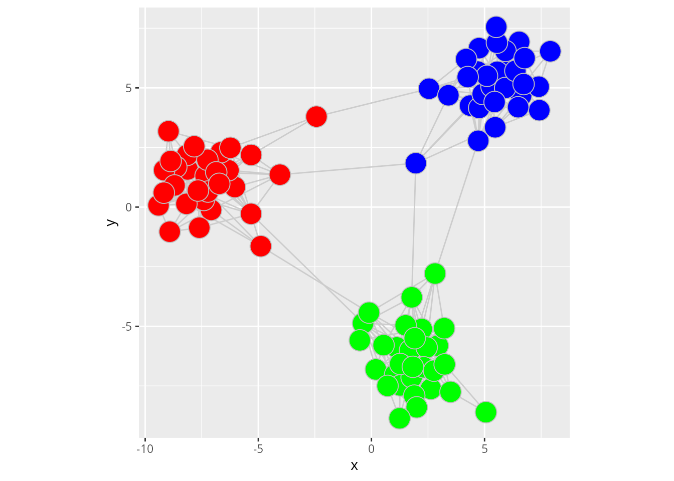

The trade-off on this approach is that, on one hand, all attributes reflect the original data directly, but no legend is accessible. This is because identity scales bypass the legend-building process of ggplot2. If a legend is required to explain the meaning of these colors, the attribute should be mapped via aesthetics (e.g., aes(fill = attribute)) and modified by a scale_*() function.

Mapping categorical variables

In this example, the node categorical variable node_group is mapped to the fill aesthetic. We call geom_edgespace() and geom_nodespace() as independent layers to provide maximum flexibility when mapping aesthetics with legends.

ggplot(gs) + geom_edgespace() +
  geom_nodespace(aes(fill = node_group), colour = "grey") +
  scale_fill_viridis_d(option = "viridis") +
  theme_gspace_coords()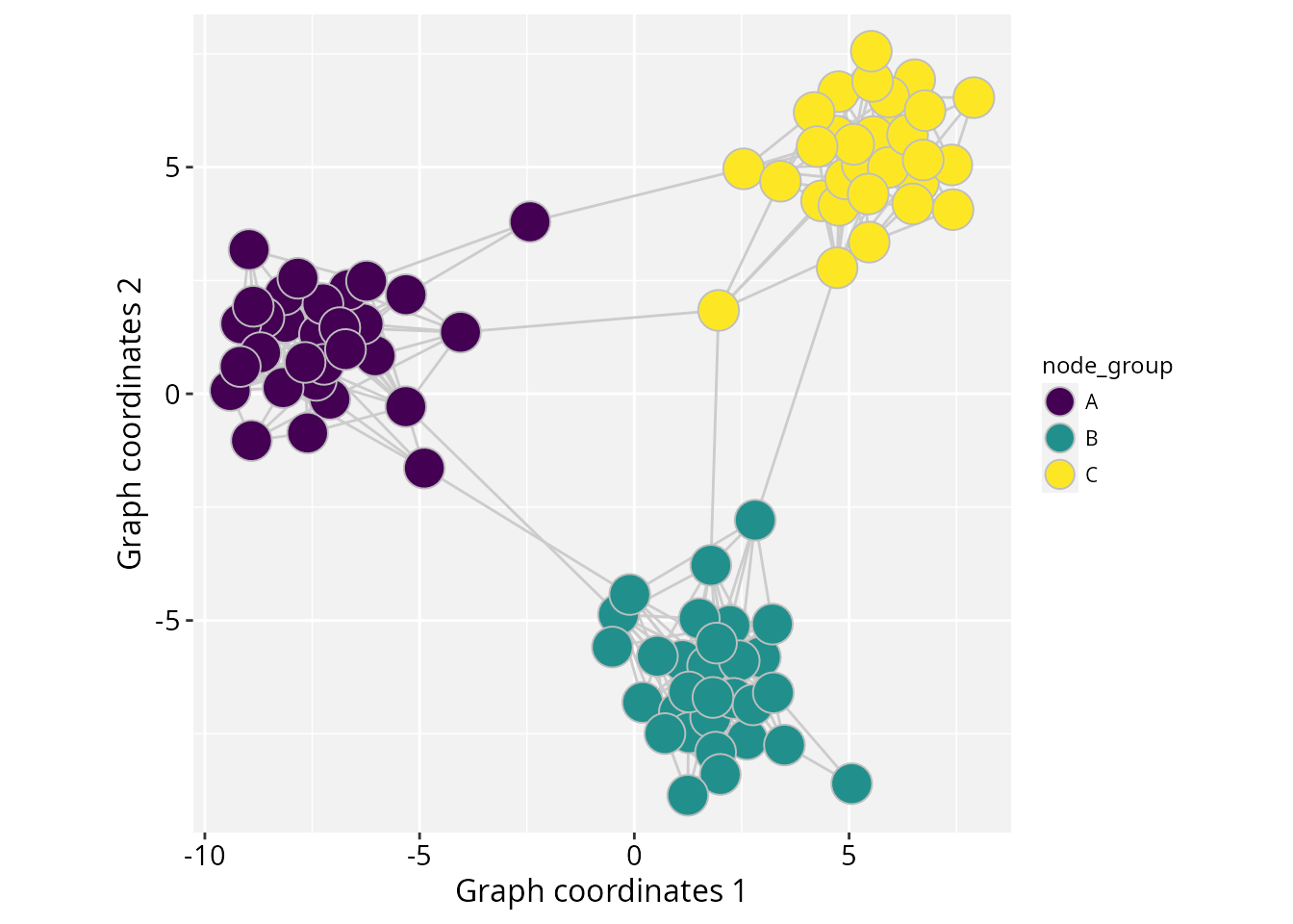

Mapping numeric variables

In this example, node and edge numeric variables are mapped to fill and colour aesthetics, respectively.

# Map aesthetics to numeric variables
ggplot(gs) + 
  geom_edgespace(aes(colour = edge_var)) +
  geom_nodespace(aes(fill = node_var), colour = "grey") +
  scale_colour_continuous(palette = c("cyan","blue")) +
  scale_fill_continuous(palette = c("white","purple")) +
  theme_gspace_coords()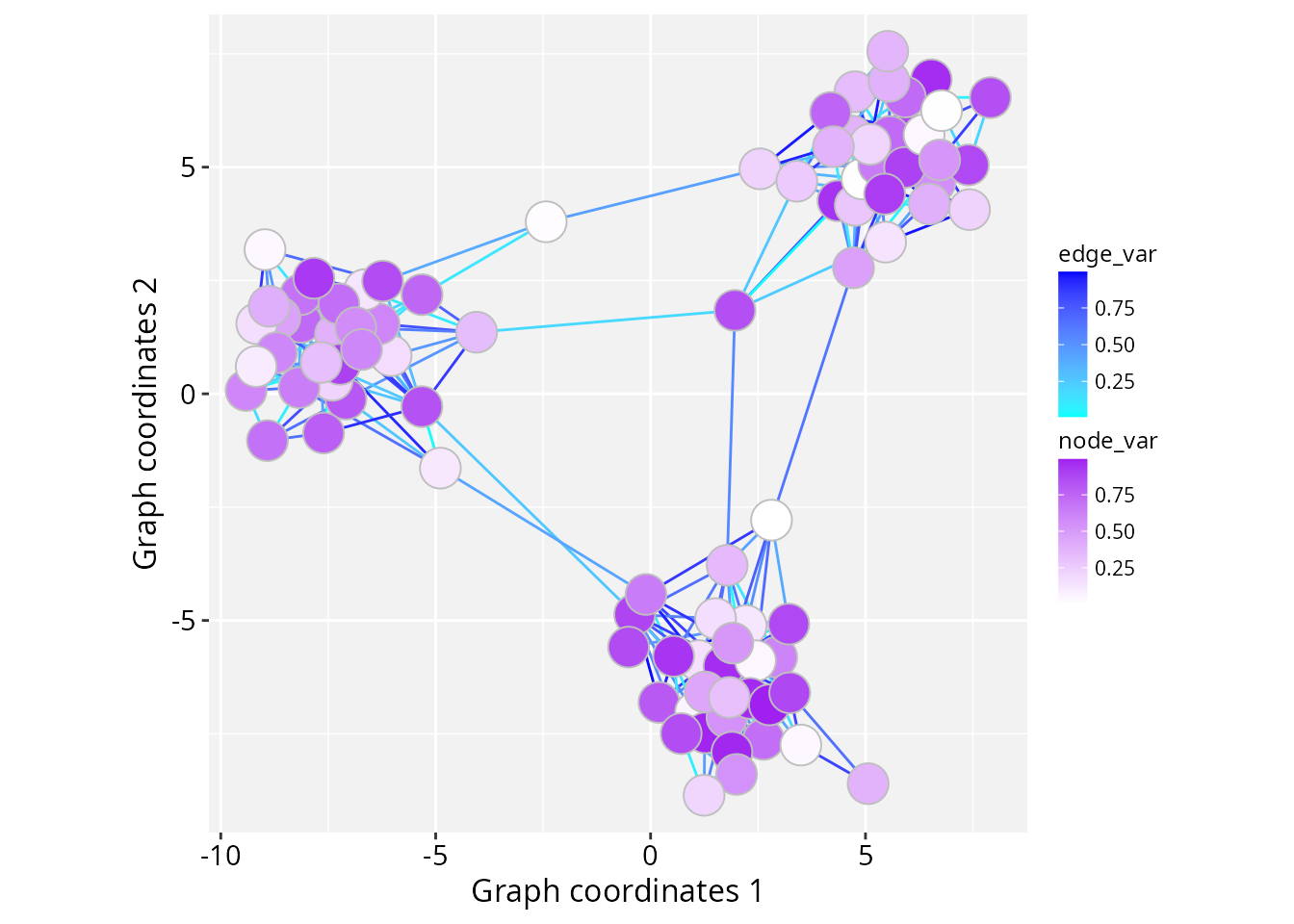

Using separate colour scales

If you need to map different variables to the same aesthetic (such as colour) with independent scales, the ggnewscale package offers an elegant solution to introduce additional scales within the same plot (Campitelli 2025); for example:

if (!require("ggnewscale", quietly = TRUE)) {
  install.packages("ggnewscale")
}
library("ggnewscale")
ggplot(data = gs) + 
  geom_edgespace(aes(colour = edge_var)) +
  scale_colour_continuous(palette = c("cyan","blue")) +
  ggnewscale::new_scale_colour() +
  geom_nodespace(aes(colour = node_var), 
    stroke = 2, fill = NA) +
  scale_colour_continuous(palette = c("white","purple")) +
  theme_gspace_coords()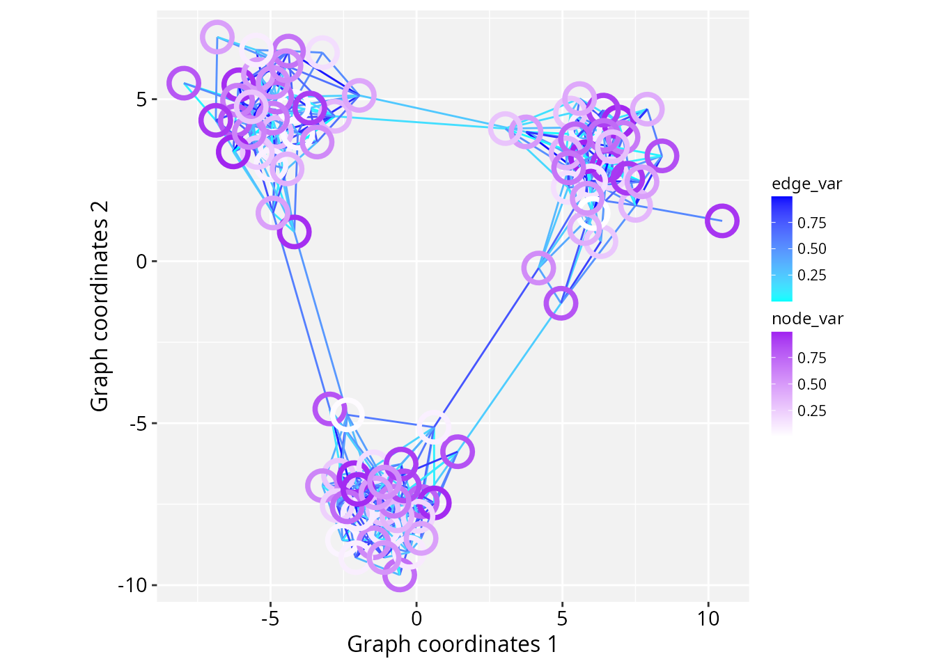

Session information

#> R version 4.6.0 (2026-04-24)
#> Platform: x86_64-pc-linux-gnu
#> Running under: Ubuntu 24.04.4 LTS
#> 
#> Matrix products: default
#> BLAS:   /usr/lib/x86_64-linux-gnu/openblas-pthread/libblas.so.3 
#> LAPACK: /usr/lib/x86_64-linux-gnu/openblas-pthread/libopenblasp-r0.3.26.so;  LAPACK version 3.12.0
#> 
#> locale:
#>  [1] LC_CTYPE=en_US.UTF-8       LC_NUMERIC=C              
#>  [3] LC_TIME=en_US.UTF-8        LC_COLLATE=en_US.UTF-8    
#>  [5] LC_MONETARY=en_US.UTF-8    LC_MESSAGES=en_US.UTF-8   
#>  [7] LC_PAPER=en_US.UTF-8       LC_NAME=C                 
#>  [9] LC_ADDRESS=C               LC_TELEPHONE=C            
#> [11] LC_MEASUREMENT=en_US.UTF-8 LC_IDENTIFICATION=C       
#> 
#> time zone: America/Sao_Paulo
#> tzcode source: system (glibc)
#> 
#> attached base packages:
#> [1] stats     graphics  grDevices utils     datasets  methods   base     
#> 
#> other attached packages:
#> [1] RGraphSpace_1.3.0 ggplot2_4.0.3     igraph_2.3.1     
#> 
#> loaded via a namespace (and not attached):
#>  [1] gtable_0.3.6       jsonlite_2.0.0     dplyr_1.2.1        compiler_4.6.0    
#>  [5] tidyselect_1.2.1   ggbeeswarm_0.7.3   tidyr_1.3.2        jquerylib_0.1.4   
#>  [9] systemfonts_1.3.2  scales_1.4.0       textshaping_1.0.5  yaml_2.3.12       
#> [13] fastmap_1.2.0      R6_2.6.1           labeling_0.4.3     generics_0.1.4    
#> [17] knitr_1.51         htmlwidgets_1.6.4  tibble_3.3.1       desc_1.4.3        
#> [21] bslib_0.10.0       pillar_1.11.1      RColorBrewer_1.1-3 rlang_1.2.0       
#> [25] cachem_1.1.0       xfun_0.57          fs_2.1.0           sass_0.4.10       
#> [29] S7_0.2.2           otel_0.2.0         viridisLite_0.4.3  cli_3.6.6         
#> [33] withr_3.0.2        pkgdown_2.2.0      magrittr_2.0.5     digest_0.6.39     
#> [37] grid_4.6.0         rstudioapi_0.18.0  beeswarm_0.4.0     lifecycle_1.0.5   
#> [41] vipor_0.4.7        ggrastr_1.0.2      vctrs_0.7.3        evaluate_1.0.5    
#> [45] glue_1.8.1         farver_2.1.2       ragg_1.5.2         tidygraph_1.3.1   
#> [49] purrr_1.2.2        rmarkdown_2.31     tools_4.6.0        pkgconfig_2.0.3   
#> [53] htmltools_0.5.9

References

Campitelli, Elio. 2025. Ggnewscale: Multiple Fill and Colour Scales in ’Ggplot2’. https://doi.org/10.32614/CRAN.package.ggnewscale.

Wickham, Hadley. 2016. Ggplot2: Elegant Graphics for Data Analysis. Springer-Verlag New York. https://ggplot2.tidyverse.org.

Sysbiolab Team

2026-05-23