Extending ggplot2 Grammar to High-Dimensional Data

Package: RGraphSpace 1.4.1

Overview

While developing RGraphSpace, the challenge of representing graph structures in ggplot2 highlighted a core design restriction: that plotting data must be expressed in tabular form, typically as a single data.frame (Wickham 2016). This approach works remarkably well for most applications, but becomes too restrictive when dealing with data objects composed of multiple interdependent components.

In this vignette, we explore how the ggplot-GraphSpace interface can be applied to high-dimensional data, enabling direct interaction with the ggplot2 grammar and its aesthetic mapping mechanisms without repeated conversion into flat tabular representations. We demonstrate this approach using the Seurat package (Hao et al. 2024). Seurat objects encapsulate multiple coordinated representations of single-cell data, making them representative examples of high-dimensional data that cannot be naturally expressed as a single data.frame.

Before you start

This vignette assumes prior experience with Seurat (Hao et al. 2024), especially for handling transcriptomics data.

Note: If you are new to Seurat, we recommend reviewing its visualization tutorials before proceeding.

Computational requirement:

Hardware: RAM >= 16 GB
Software: R (>=4.5) and RStudio

Required packages

Before proceeding, ensure that all packages described in the Installation Instructions are installed.

# Check versions
if (packageVersion("RGraphSpace") < "1.4.1"){
  message("Need to update 'RGraphSpace' for this vignette")
  remotes::install_github("sysbiolab/RGraphSpace")
}
if (packageVersion("Seurat") < "5.5.0"){
  message("Need to update 'Seurat' for this vignette")
  remotes::install_github("satijalab/Seurat")
}

Setting input data

# Load packages
library("RGraphSpace")
library("Seurat")
library("SeuratObject")
library("SeuratData")
library("patchwork")

Loading the dataset

We will use the pbmc3k dataset from the SeuratData package, consisting of single-cell transcriptomics data from peripheral blood mononuclear cells. This dataset is commonly used to showcase Seurat workflows (Hao et al. 2024).

# Install a Seurat dataset (required only once)
SeuratData::InstallData("pbmc3k")

# Check manifest of installed datasets
# SeuratData::InstalledData()

# Load the 'pbmc3k' dataset
# Note: LoadData() may print conversion warnings when loading pbmc3k.
# These are expected and come from SeuratData's internal v4-to-v5
# object migration — they can be safely ignored.
seurat_obj <- LoadData("pbmc3k", type = "pbmc3k.final")

## Common Seurat preprocessing workflow.
## Shown for reference only, as the 'pbmc3k' 
## dataset has already been preprocessed.
# seurat_obj <- NormalizeData(seurat_obj)
# seurat_obj <- ScaleData(seurat_obj)
# seurat_obj <- FindVariableFeatures(seurat_obj)
# seurat_obj <- RunPCA(seurat_obj)
# seurat_obj <- RunUMAP(seurat_obj, dims = 1:30)

Seurat reference plots

Before introducing the ggplot-GraphSpace interface, we first reproduce two typical Seurat visualizations: a cluster-level embedding (DimPlot) and a feature expression map (FeaturePlot). These examples provide a useful baseline for the corresponding visualizations constructed later with ggplot-GraphSpace.

cpal <- DiscretePalette(nlevels(seurat_obj$seurat_annotations), 
  palette = "polychrome")

# Left: cluster-level embedding
p1 <- DimPlot(seurat_obj, pt.size = 1, cols = cpal) + 
  theme_minimal() + theme(aspect.ratio = 1)
p1

# Right: feature expression map
p2 <- FeaturePlot(seurat_obj, features = "LYZ", 
  cols = c("lightgrey", "blue"), pt.size = 1) + 
  theme_minimal() + theme(aspect.ratio = 1)
p2

# Plot side-by-side
# p1 + p2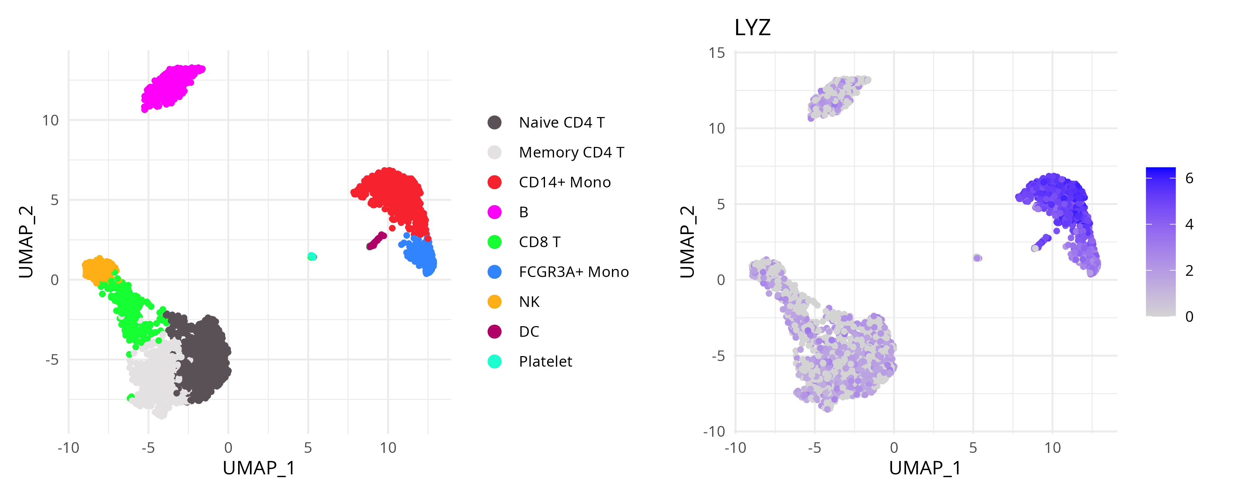

Note that DimPlot and FeaturePlot are high-level functions. Internally, Seurat extracts the relevant data and generates ggplot objects. While convenient, the underlying data structures are not directly exposed to the user, making advanced use of the ggplot2 grammar more difficult. For example, defining custom aesthetic mappings or interoperating with other visualization workflows would require extra data extraction steps.

Exposing the ggplot2 grammar

We now apply as.GraphSpace() to expose the Seurat object’s underlying high-dimensional data directly to ggplot2 (for additional details, see the coercing high-dimensional data section).

# Create a GraphSpace from 'seurat_obj'
gs <- as.GraphSpace(seurat_obj, space = "embedding", reduction = "umap")

# Seurat object converted to GraphSpace:
# ℹ space=embedding, layer=default, features=13714, samples=2638, reduction="umap"
# Node spatial boundaries:
# ℹ x: [-9, 13] (cols)
# ℹ y: [-9, 14] (rows)

gs
# A GraphSpace-class object for:
# IGRAPH 1393201 UN-- 2638 0 -- 
# + attr: x (v/n), y (v/n), name (v/c), nodeLabel (v/c), nodeSize (v/n), orig.ident (v/x),
# | nCount_RNA (v/n), nFeature_RNA (v/n), seurat_annotations (v/x), percent.mt (v/n),
# | RNA_snn_res.0.5 (v/x), seurat_clusters (v/x), arrowType (e/n)
# + features: 13714 (AL627309.1, AP006222.2, RP11-206L10.2, RP11-206L10.9, ...)

With the GraphSpace object ready, we reproduce the same plots using ggplot2 geoms and aesthetic mappings.

cpal <- DiscretePalette(nlevels(gs$seurat_annotations), 
  palette = "polychrome")

# Left: cluster-level embedding
p3 <- ggplot(gs) + 
  geom_nodespace(mapping = aes(fill = seurat_annotations),
    size = 1.5, color = "grey90", stroke = 0.3) +
  scale_fill_manual(values = cpal) +
  labs(x = "UMAP_1", y = "UMAP_2") +
  theme_gspace_legend(discrete_fill = TRUE) +
  theme_minimal() + theme(aspect.ratio = 1)
p3

# Right: feature expression map
p4 <- ggplot(gs) + 
  geom_nodespace(mapping = aes(fill = LYZ), 
    size = 1.5, color = "lightgrey", stroke = 0.3) +
  scale_fill_continuous(palette = c("lightgrey", "blue")) +
  labs(x = "UMAP_1", y = "UMAP_2")  +
  theme_minimal() + theme(aspect.ratio = 1)
p4

# Plot side-by-side
# p3 + p4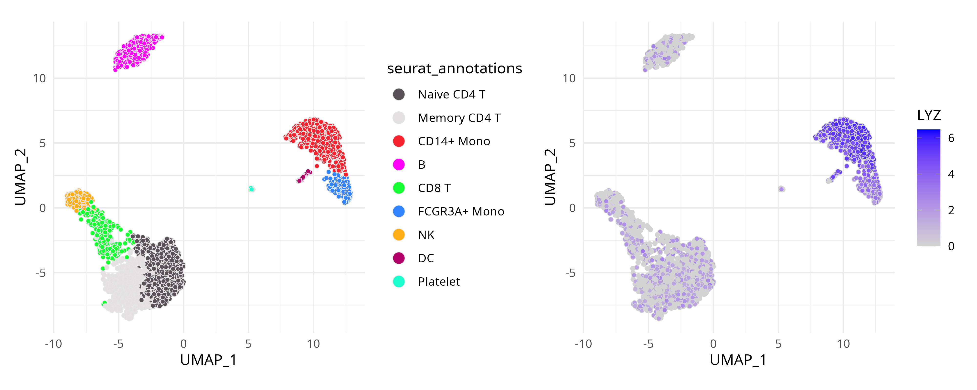

The resulting plots are essentially the same, but users now have full flexibility to interact directly with ggplot2 and its rich ecosystem of extensions and companion packages.

Coercing high-dimensional data

The as.GraphSpace() function provides a convenient way to coerce high-dimensional data into a GraphSpace object. However, no coercion method can anticipate every possible data structure. Below, we show how to access the relevant components of a Seurat object and use them to construct a GraphSpace manually. For another coercion example, see the spatial data tutorial.

# Extract UMAP embeddings as node coordinates
coords <- Embeddings(seurat_obj, reduction = "umap")
coords <- coords[, seq_len(2)] |> as.data.frame()
colnames(coords) <- c("x", "y")

# Extract cell metadata
metadata <- seurat_obj[[]]

# Merge coordinates and metadata using common cell identifiers
ids <- intersect(rownames(coords), rownames(metadata))
coords <- cbind(coords[ids, ], metadata[ids, ])

# Construct a GraphSpace object
# Metadata become node attributes
gs <- GraphSpace(coords)

# Add high-dimensional feature data
# Stored separately for lazy aesthetic mapping
gs_fdata(gs) <- SeuratObject::LayerData(seurat_obj, layer = "data")

# Optional: normalize node coordinates
gs <- normalizeGraphSpace(gs, mar = 0.01)

Session information

#> R version 4.6.0 (2026-04-24)
#> Platform: x86_64-pc-linux-gnu
#> Running under: Ubuntu 24.04.4 LTS
#> 
#> Matrix products: default
#> BLAS:   /usr/lib/x86_64-linux-gnu/openblas-pthread/libblas.so.3 
#> LAPACK: /usr/lib/x86_64-linux-gnu/openblas-pthread/libopenblasp-r0.3.26.so;  LAPACK version 3.12.0
#> 
#> locale:
#>  [1] LC_CTYPE=en_US.UTF-8       LC_NUMERIC=C              
#>  [3] LC_TIME=en_US.UTF-8        LC_COLLATE=en_US.UTF-8    
#>  [5] LC_MONETARY=en_US.UTF-8    LC_MESSAGES=en_US.UTF-8   
#>  [7] LC_PAPER=en_US.UTF-8       LC_NAME=C                 
#>  [9] LC_ADDRESS=C               LC_TELEPHONE=C            
#> [11] LC_MEASUREMENT=en_US.UTF-8 LC_IDENTIFICATION=C       
#> 
#> time zone: America/Sao_Paulo
#> tzcode source: system (glibc)
#> 
#> attached base packages:
#> [1] stats     graphics  grDevices utils     datasets  methods   base     
#> 
#> other attached packages:
#>  [1] patchwork_1.3.2           stxBrain.SeuratData_0.1.2
#>  [3] ssHippo.SeuratData_3.1.4  pbmc3k.SeuratData_3.1.4  
#>  [5] SeuratData_0.2.2.9002     Seurat_5.5.0             
#>  [7] SeuratObject_5.4.0        sp_2.2-1                 
#>  [9] RGraphSpace_1.4.1         ggplot2_4.0.3            
#> 
#> loaded via a namespace (and not attached):
#>   [1] RColorBrewer_1.1-3     rstudioapi_0.18.0      jsonlite_2.0.0        
#>   [4] magrittr_2.0.5         spatstat.utils_3.2-3   ggbeeswarm_0.7.3      
#>   [7] farver_2.1.2           rmarkdown_2.31         fs_2.1.0              
#>  [10] ragg_1.5.2             vctrs_0.7.3            ROCR_1.0-12           
#>  [13] spatstat.explore_3.8-1 htmltools_0.5.9        sass_0.4.10           
#>  [16] sctransform_0.4.3      parallelly_1.47.0      KernSmooth_2.23-26    
#>  [19] bslib_0.11.0           htmlwidgets_1.6.4      desc_1.4.3            
#>  [22] ica_1.0-3              fontawesome_0.5.3      plyr_1.8.9            
#>  [25] plotly_4.12.0          zoo_1.8-15             cachem_1.1.0          
#>  [28] igraph_2.3.2           mime_0.13              lifecycle_1.0.5       
#>  [31] pkgconfig_2.0.3        Matrix_1.7-5           R6_2.6.1              
#>  [34] fastmap_1.2.0          fitdistrplus_1.2-6     future_1.70.0         
#>  [37] shiny_1.13.0           digest_0.6.39          tensor_1.5.1          
#>  [40] RSpectra_0.16-2        irlba_2.3.7            textshaping_1.0.5     
#>  [43] progressr_0.19.0       spatstat.sparse_3.2-0  httr_1.4.8            
#>  [46] polyclip_1.10-7        abind_1.4-8            compiler_4.6.0        
#>  [49] withr_3.0.2            S7_0.2.2               fastDummies_1.7.6     
#>  [52] MASS_7.3-65            rappdirs_0.3.4         tools_4.6.0           
#>  [55] vipor_0.4.7            lmtest_0.9-40          otel_0.2.0            
#>  [58] beeswarm_0.4.0         httpuv_1.6.17          future.apply_1.20.2   
#>  [61] goftest_1.2-3          glue_1.8.1             nlme_3.1-169          
#>  [64] promises_1.5.0         grid_4.6.0             Rtsne_0.17            
#>  [67] cluster_2.1.8.2        reshape2_1.4.5         generics_0.1.4        
#>  [70] gtable_0.3.6           spatstat.data_3.1-9    tidyr_1.3.2           
#>  [73] data.table_1.18.4      tidygraph_1.3.1        spatstat.geom_3.8-1   
#>  [76] RcppAnnoy_0.0.23       ggrepel_0.9.8          RANN_2.6.2            
#>  [79] pillar_1.11.1          stringr_1.6.0          spam_2.11-4           
#>  [82] RcppHNSW_0.7.0         later_1.4.8            splines_4.6.0         
#>  [85] dplyr_1.2.1            lattice_0.22-9         survival_3.8-6        
#>  [88] deldir_2.0-4           tidyselect_1.2.1       miniUI_0.1.2          
#>  [91] pbapply_1.7-4          knitr_1.51             gridExtra_2.3         
#>  [94] scattermore_1.2        xfun_0.58              matrixStats_1.5.0     
#>  [97] stringi_1.8.7          lazyeval_0.2.3         yaml_2.3.12           
#> [100] evaluate_1.0.5         codetools_0.2-20       tibble_3.3.1          
#> [103] cli_3.6.6              uwot_0.2.4             xtable_1.8-8          
#> [106] reticulate_1.46.0      systemfonts_1.3.2      jquerylib_0.1.4       
#> [109] Rcpp_1.1.1-1.1         globals_0.19.1         spatstat.random_3.5-0 
#> [112] png_0.1-9              ggrastr_1.0.2          spatstat.univar_3.2-0 
#> [115] parallel_4.6.0         pkgdown_2.2.0          dotCall64_1.2         
#> [118] listenv_0.10.1         viridisLite_0.4.3      scales_1.4.0          
#> [121] ggridges_0.5.7         crayon_1.5.3           purrr_1.2.2           
#> [124] rlang_1.2.0            cowplot_1.2.0

Hao, Yuhan, Tim Stuart, Madeline H Kowalski, et al. 2024. “Dictionary Learning for Integrative, Multimodal and Scalable Single-Cell Analysis.” Nature Biotechnology 42 (2): 293–304. https://doi.org/10.1038/s41587-023-01767-y.

Wickham, Hadley. 2016. Ggplot2: Elegant Graphics for Data Analysis. Springer-Verlag New York. https://ggplot2.tidyverse.org.

Sysbiolab Team

2026-06-23