Mapping Graphs to Images
Sysbiolab Team
2026-10-19
Source:vignettes/articles/mapping-images.Rmd
mapping-images.Rmd
Package: RGraphSpace 1.5.7
# Check required version
if (packageVersion("RGraphSpace") < "1.5.7"){
  message("Need to update 'RGraphSpace' for this vignette")
  remotes::install_github("sysbiolab/RGraphSpace")
}
Overview
Images can be used as spatial references for graphs. When a raster image is provided, the pixel coordinates define where nodes are positioned, supporting the construction of graphs from image features. However, spatial alignment requires consistent coordinate conventions between the graph and the image; a mismatch in axis orientation, for example a top-left versus bottom-left origin, leaves the nodes reflected relative to the image.
Graph and image conventions
We begin with a simple toy example that highlights how graphs and images follow different conventions and need to be transformed into the same coordinate space for layered visualization. This toy illustrates a scenario in which the image registration has already been performed (see image registration section), with graph nodes representing image features.
library("RGraphSpace")
library("igraph")
library("ggplot2")
library("patchwork")

# Load a toy GraphSpace object, which already
# includes an embedded image, with node
# coordinates mapping to image indices.
data("gs_image_toy")

# Check node and image spatial boundaries
gs_image_toy
#> A GraphSpace-class object for:
#> IGRAPH 2a25533 DN-- 5 4 --
#> + attr: x (v/n), y (v/n), name (v/c), nodeLabel (v/c), nodeLabelColor
#> | (v/c), nodeSize (v/n), edgeColor (e/c), arrowType (e/n)
#> + node payload: 1 (nodeFillColor)
#> + node spatial boundaries: raw graph
#> | x: [194, 493] (cols)
#> | y: [237, 412] (rows)
#> + image spatial boundaries: raw image
#> | x: [1, 680] (cols)
#> | y: [1, 640] (rows)
Node coordinates fall within the image’s spatial boundaries: nodes
range x:[194, 493](cols) and
y:[237, 412](rows), while the image spans
x:[1, 680](cols) and y:[1, 640](rows),
consistent with a common frame of reference. The image is composed of
several amorphous shapes and a bluish feature region to which the graph
nodes are registered. A red node is included to break visual symmetry,
and a corresponding reddish mark in the feature region allows its
position to be tracked against the image.
# Plot the un-normalized image
p1 <- ggplot() +
  annotation_gspace_image(gs_image_toy) +
  scale_x_continuous(name = "Image coordinates 1", limits = c(0, 1)) +
  scale_y_continuous(name = "Image coordinates 2", limits = c(0, 1)) +
  theme(aspect.ratio = 1)

# Plot the un-normalized graph
p2 <- ggplot(gs_image_toy) +
  geom_edgespace() + geom_nodespace() +
  scale_x_continuous(name = "Graph coordinates 1", limits = c(190, 500)) +
  scale_y_continuous(name = "Graph coordinates 2", limits = c(190, 500)) +
  theme(aspect.ratio = 1)

p1 + p2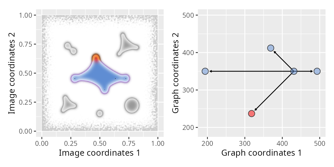
When rendered as separate plots, the image spans [0,1],
while the graph spans ~[190, 500]; these are different
coordinate spaces entirely, so a simple merge would misplace them. A
separate mismatch is orientation: the red node and its corresponding
reddish mark in the feature region show that the image is rendered
top-down, while the graph is rendered bottom-up.
Next, normalizeGraphSpace() maps node coordinates to
image space and converts the source image into a render-ready canvas. By
default, it flips node y-coordinates over the image center to match the
image’s orientation, then crops the image to the graph’s extent (plus a
margin), so that the resulting canvas is centered on the graph.
gs_image_toy <- normalizeGraphSpace(gs_image_toy, mar = 0.1)
#> Normalizing node coordinates to image space...
#> Flipping y-coordinates over image center...

ggplot(gs_image_toy) +
  annotation_gspace_image(gs_image_toy) +
  geom_edgespace() + geom_nodespace() +
  theme_gspace_coords(is_norm = TRUE)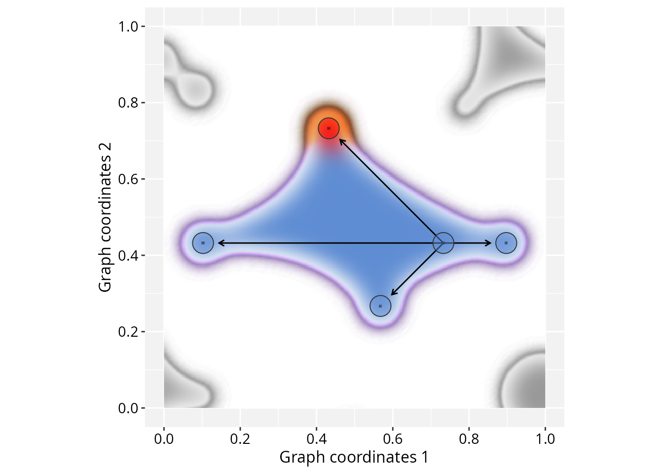
The default mar = 0.1 leaves a margin of
0.1 on each side, so the graph occupies the central
0.8 of the canvas.
For reference, here is the result when no flip is applied to node coordinates:
gs_image_toy <- normalizeGraphSpace(gs_image_toy, flip.y = FALSE)
#> Normalizing node coordinates to image space...

ggplot(gs_image_toy) +
  annotation_gspace_image(gs_image_toy) +
  geom_edgespace() + geom_nodespace() +
  theme_gspace_coords(is_norm = TRUE)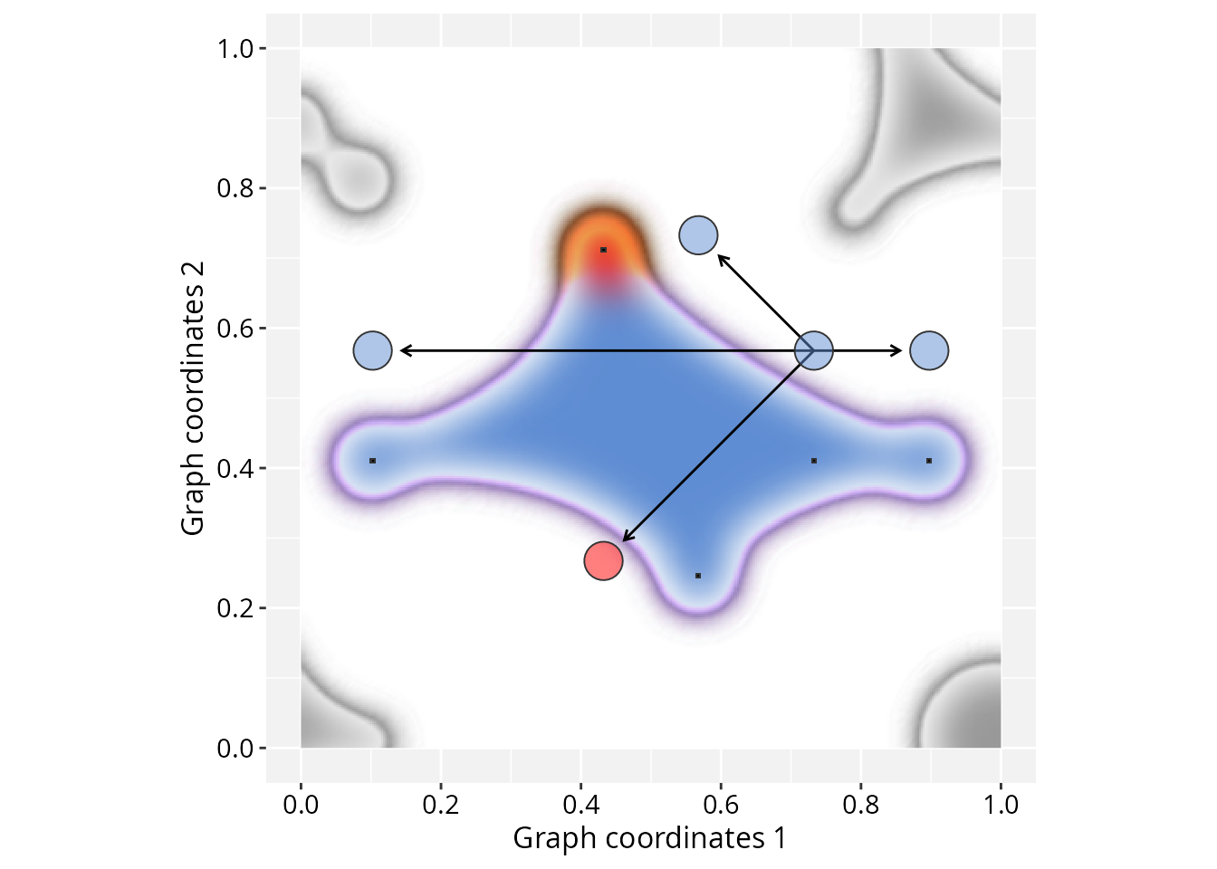
Note on image alignment: Spatial misalignment may
occur if the input image and node coordinates differ in axis orientation
(e.g., top-left versus bottom-left origins). To accommodate these
differences, normalizeGraphSpace() provides orientation
controls through the swap.xy, flip.x, and
flip.y arguments. If the nodes appear misaligned with the
input image, try combinations of these parameters to correct the
alignment. Alternatively, try flip.v and
flip.h arguments to apply flipping directly to the
background image (see the orientation controls subsection)
Image registration
Image registration is a broad field concerned with estimating a spatial transformation that aligns a query to a reference dataset (Lewis et al. 2021; Balluff et al. 2022). RGraphSpace addresses a special case where the spatial correspondence between graph and image is known by construction, so the alignment task reduces to correcting axis-orientation mismatches, fixing node positions to their target pixels, and normalizing graph and image to a common coordinate space. In this section we exemplify this constrained workflow by extracting pixel coordinates from an image matrix and building a graph with nodes placed at those positions.
Setting basic input data
Next, we extract pixel coordinates at a specific intensity quantile
from the volcano matrix and prepare an igraph
for RGraphSpace.
library("RGraphSpace")
library("igraph")
library("ggplot2")

# Extract pixel coordinates for a specific intensity quantile.
coords <- which(volcano == quantile(volcano, 0.85), arr.ind = TRUE)

# Mark target pixels with '0'; it will appear as black in the background.
# This creates a visual anchor to verify the alignment precision.
volcano2 <- volcano
volcano2[coords] <- 0

# Create an igraph object from the pixel coordinates;
# note that at this stage, 'y' represents matrix row indices.
gtoy3 <- igraph::make_empty_graph(n = nrow(coords))
igraph::V(gtoy3)$y <- coords[,1]
igraph::V(gtoy3)$x <- coords[,2]

# Highlight the bottom-row vertex (max 'y' index) to demonstrate alignment;
# since matrix indexing is top-down, this accounts for the default flip
# between matrix and plot coordinate systems.
igraph::V(gtoy3)$nodeFillColor <- NA
bottom_row <- which.max(igraph::V(gtoy3)$y)
igraph::V(gtoy3)$nodeFillColor[bottom_row] <- adjustcolor("red", 0.4)
Initialize, normalize, and plot
# Initialize a GraphSpace object
gs <- GraphSpace(gtoy3)
#> Validating the 'igraph' object...
#> Vertex attribute 'name' missing; assigning names...
#> Creating a 'GraphSpace' object...

# Add a raster image
gs_image(gs) <- as_colorraster(volcano2)

# Map graph coordinates to the image space; by default,
# y-coordinates will be flipped (see comments below).
gs <- normalizeGraphSpace(gs)
#> Normalizing node coordinates to image space...
#> Flipping y-coordinates over image center...

gs
#> A GraphSpace-class object for:
#> IGRAPH 59db705 DN-- 39 0 --
#> + attr: x (v/n), y (v/n), name (v/c), nodeLabel (v/c), nodeSize (v/n),
#> | nodeFillColor (v/c), arrowType (e/c)
#> + node spatial boundaries: normalized to image space
#> | x: [16, 50] -> [0, 1] (cols)
#> | y: [11, 51] -> [0, 1] (rows)
#> + image spatial boundaries: cropped to graph space
#> | x: [1, 61] -> [1, 51] (cols)
#> | y: [1, 87] -> [1, 51] (rows)
Observe that the nodes (open circles) are precisely aligned with the pixels (dark squares) to which they were mapped. In this plot, nodes remain proportional to the viewport regardless of the final output resolution. This behavior is especially critical when the network elements represent image features at specific positions and must stay anchored to those features, avoiding overlap with adjacent, unrelated areas.
# Render the graph with the raster as background
plotGraphSpace(gs, add.image = TRUE)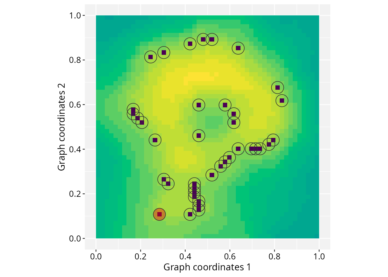
# Alternatively, passing to the underlying geoms
ggplot(gs) +
  annotation_gspace_image(gs) +
  geom_nodespace() +
  theme_gspace_coords(is_norm = TRUE)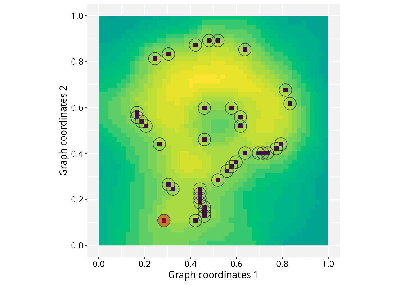
Orientation controls
The normalizeGraphSpace() function provides five
arguments to adjust the alignment between graph coordinates and the
background image. Arguments flip.x, flip.y,
and swap.xy transform node coordinates; flip.v
and flip.h transform the image matrix itself. The reference
card below illustrates each argument using the volcano
dataset, where nodes are precisely aligned with their corresponding dark
pixels in the default configuration. Each panel shows how that alignment
changes when a single argument is modified.
Note that flip.y defaults to TRUE when
image.space = TRUE, since image matrices use a top-down row
indexing that is the inverse of the standard graph coordinate system.
The panel labelled flip.y = FALSE shows what happens when
this default correction is suppressed.
library("patchwork")

# Helper: build and render one panel
make_panel <- function(..., title) {
  gs <- GraphSpace(gtoy3)
  gs_image(gs) <- as_colorraster(volcano2)
  gs <- normalizeGraphSpace(gs, image.space = TRUE, ...)
  plotGraphSpace(gs, add.image = TRUE) +
    ggplot2::labs(title = title) +
    ggplot2::theme(
      plot.title = element_text(
        size = 12, hjust = 0.5, face = "plain"),
      plot.margin = ggplot2::margin(1, 1, 10, 1)
    )
}

# One panel per orientation argument
p1 <- make_panel(title = "default")
p2 <- make_panel(flip.x  = TRUE,  title = "flip.x = TRUE")
p3 <- make_panel(flip.y  = FALSE, title = "flip.y = FALSE")
p4 <- make_panel(swap.xy = TRUE,  title = "swap.xy = TRUE")
p5 <- make_panel(flip.v  = TRUE,  title = "flip.v = TRUE")
p6 <- make_panel(flip.h  = TRUE,  title = "flip.h = TRUE")

# 3x2 reference grid
(p1 | p2 | p3) / (p4 | p5 | p6)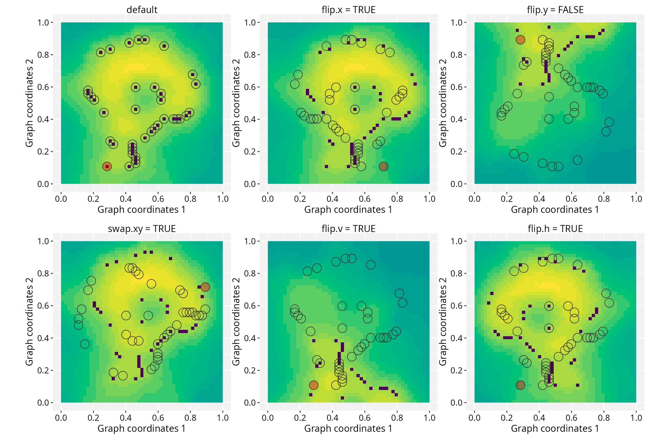
Advanced workflows
See the Spatial Data tutorial for examples using a reference image.
Session information
#> R version 4.6.1 (2026-06-24)
#> Platform: x86_64-pc-linux-gnu
#> Running under: Ubuntu 24.04.5 LTS
#>
#> Matrix products: default
#> BLAS:   /usr/lib/x86_64-linux-gnu/openblas-pthread/libblas.so.3
#> LAPACK: /usr/lib/x86_64-linux-gnu/openblas-pthread/libopenblasp-r0.3.26.so;  LAPACK version 3.12.0
#>
#> locale:
#>  [1] LC_CTYPE=en_US.UTF-8       LC_NUMERIC=C
#>  [3] LC_TIME=en_US.UTF-8        LC_COLLATE=en_US.UTF-8
#>  [5] LC_MONETARY=en_US.UTF-8    LC_MESSAGES=en_US.UTF-8
#>  [7] LC_PAPER=en_US.UTF-8       LC_NAME=C
#>  [9] LC_ADDRESS=C               LC_TELEPHONE=C
#> [11] LC_MEASUREMENT=en_US.UTF-8 LC_IDENTIFICATION=C
#>
#> time zone: America/Sao_Paulo
#> tzcode source: system (glibc)
#>
#> attached base packages:
#> [1] stats     graphics  grDevices utils     datasets  methods   base
#>
#> other attached packages:
#> [1] patchwork_1.3.2   igraph_2.3.4      RGraphSpace_1.5.7 ggplot2_4.0.3
#>
#> loaded via a namespace (and not attached):
#>  [1] sass_0.4.10        generics_0.1.4     tidyr_1.3.2        lattice_0.23-1
#>  [5] digest_0.6.39      magrittr_2.0.5     evaluate_1.0.5     grid_4.6.1
#>  [9] RColorBrewer_1.1-3 fastmap_1.2.0      jsonlite_2.0.0     Matrix_1.7-6
#> [13] ggrastr_1.0.2      purrr_1.2.2        scales_1.4.0       textshaping_1.0.5
#> [17] jquerylib_0.1.4    cli_3.6.6          rlang_1.3.0        tidygraph_1.3.1
#> [21] withr_3.0.3        cachem_1.1.0       yaml_2.3.12        otel_0.2.0
#> [25] ggbeeswarm_0.7.3   tools_4.6.1        dplyr_1.2.1        vctrs_0.7.3
#> [29] R6_2.6.1           lifecycle_1.0.5    fs_2.1.0           htmlwidgets_1.6.4
#> [33] vipor_0.4.7        ragg_1.5.2         pkgconfig_2.0.3    beeswarm_0.4.0
#> [37] desc_1.4.3         pkgdown_2.2.0      pillar_1.11.1      bslib_0.11.0
#> [41] gtable_0.3.6       glue_1.8.1         systemfonts_1.3.2  xfun_0.59
#> [45] tibble_3.3.1       tidyselect_1.2.1   rstudioapi_0.19.0  knitr_1.51
#> [49] dichromat_2.0-1    farver_2.1.2       htmltools_0.5.9    labeling_0.4.3
#> [53] rmarkdown_2.32     compiler_4.6.1     S7_0.2.2