Interoperability with 'ggraph' and 'sf'
Sysbiolab Team
2026-07-20
Source:vignettes/articles/interoperability.Rmd
interoperability.Rmd
Package: RGraphSpace 1.4.4
Overview
RGraphSpace is designed to be a seamless extension to
existing network analysis workflows, not a replacement. Whether using
igraph (Csardi and Nepusz 2006)
for heavy-duty computations or tidygraph (Pedersen 2025) for tidy data manipulation,
RGraphSpace geoms automatically recognize these
objects on the fly. The main motivation behind RGraphSpace was
to address the challenge of scaling network elements without disrupting
alignment with image features. For practical examples, see mapping graphs to images; see
also PathwaySpace
tutorials for use-case scenarios involving reference image
backgrounds.
Why use RGraphSpace with ggraph?
While ggraph is a wonderful framework for relational data,
precise edge-node alignment requires additional handling when node sizes
vary dynamically. This limitation arises from a fundamental trade-off in
ggplot2: scaling size aesthetic is tied to a fixed
physical legend representation, causing node dimensions to depend on
device scaling rather than the normalized coordinate space. For most
applications this is not an issue, but it becomes critical when graphs
must be spatially aligned with reference images. RGraphSpace
addresses this through specialized geoms that automatically
compensate for alignment shifts introduced by node scaling. The
trade-off for this higher level of automation is that the user has fewer
customization options compared to the ggraph approach. This is
exactly why using RGraphSpace alongside ggraph makes
sense: it provides precise spatial alignment between graph elements and
reference frames while preserving interoperability with the extensive
layout and styling flexibility of the ggraph grammar.
Required packages
Before proceeding, ensure that all packages described in the Installation Instructions are installed.
# Check required version
if (packageVersion("RGraphSpace") < "1.4.3"){
  message("Need to update 'RGraphSpace' for this vignette")
  remotes::install_github("sysbiolab/RGraphSpace")
}
# Load packages
library("RGraphSpace")
library("igraph")
library("sf")
library("maps")
library("geometry")
library("tidygraph")
library("ggraph")
Setting basic input data
The following example demonstrates the interoperability between
RGraphSpace and ggraph using both igraph and
tidygraph objects, and managing spatial data with sf,
the standard infrastructure for spatial data analysis in R
(Pebesma and Bivand 2023). Integrating
network structures with spatial data often creates a headache with
mismatched coordinate systems and scales, which makes this example
particularly interesting to showcase how these packages handle that
complexity.
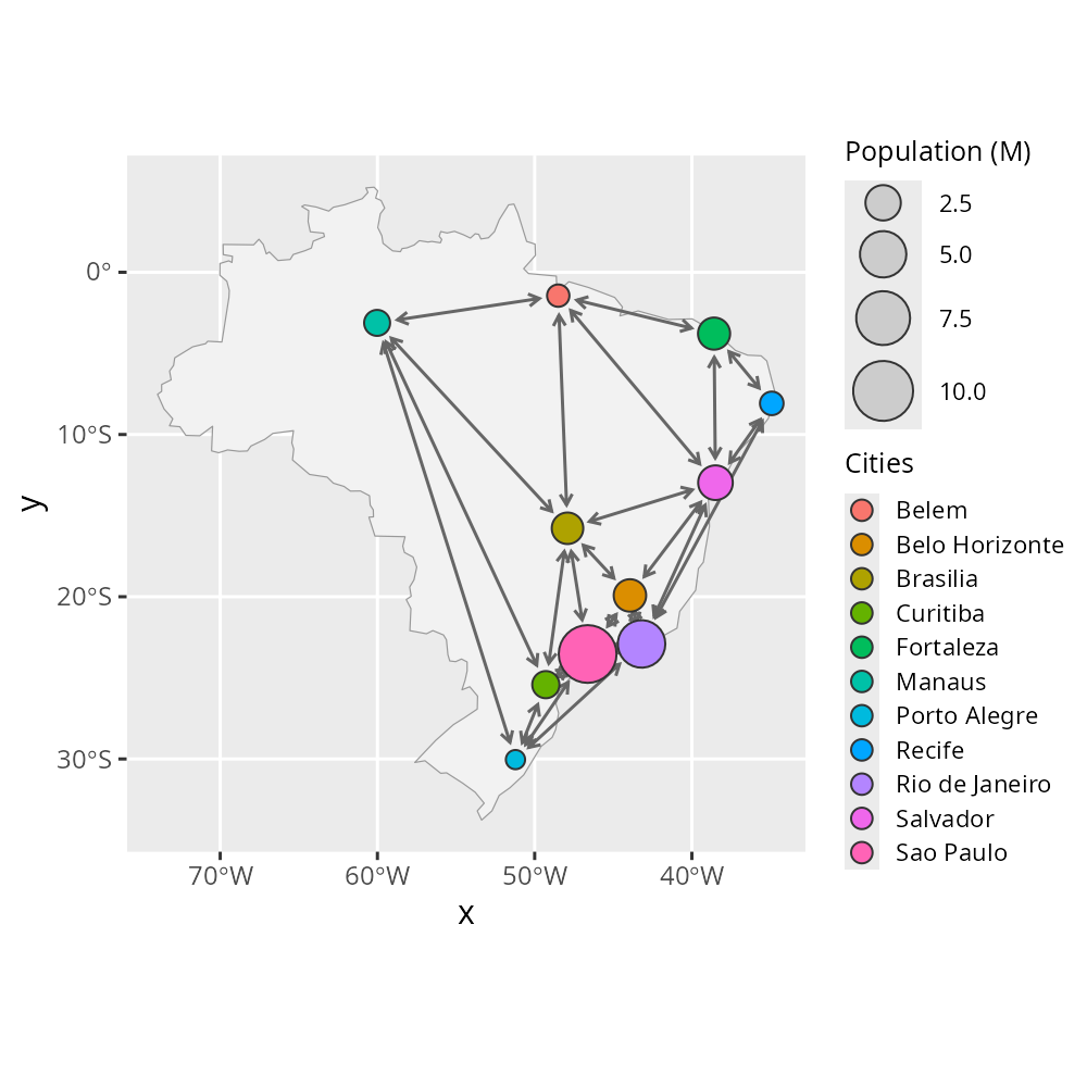
Next, we build a spatial network of cities; then RGraphSpace
geoms are plugged into ggraph and sf
workflows.
# Load a map and transform projection
map_sf <- st_as_sf(map("world", regions = "Brazil", fill = TRUE))

# Filter major cities by regional capitals
data(world.cities, package = "maps")
r_capitals <- c(
  "Aracaju", "Belem", "Belo Horizonte", "Boa Vista", "Brasilia",
  "Campo Grande", "Cuiaba", "Curitiba", "Florianopolis", "Fortaleza",
  "Goiania", "Joao Pessoa", "Macapa", "Maceio", "Manaus", "Natal",
  "Palmas", "Porto Alegre", "Porto Velho", "Recife", "Rio Branco",
  "Rio de Janeiro", "Salvador", "Sao Luis", "Sao Paulo", "Teresina",
  "Vitoria"
)
cities <- subset(world.cities, country.etc == "Brazil" &
    name %in% r_capitals & pop > 1200000)

# Create Delaunay triangulation edges
# Note: the edges hold no particular meaning beyond
# demonstrating integration between coordinate systems
tri <- delaunayn(cities[,c("lat","long")])
edges <- unique(rbind(tri[,c(1,2)], tri[,c(2,3)], tri[,c(1,3)] ))

# Build an 'igraph' using city coordinates
igraph_cities <- igraph::graph_from_edgelist(edges, directed = FALSE)
igraph::V(igraph_cities)$x <- cities$long
igraph::V(igraph_cities)$y <- cities$lat
igraph::V(igraph_cities)$Cities <- cities$name
igraph::V(igraph_cities)$`Population (M)` <- cities$pop/1000000
igraph::E(igraph_cities)$arrowType <- 3
Different input, same output
The following options all produce the same visual output, demonstrating how these packages integrate different types of input data.
# Option 1: Passing a 'GraphSpace' object directly to ggplot()
gs <- GraphSpace(igraph_cities)
ggplot(gs) +
  geom_sf(data = map_sf, fill = "grey95", color = "grey60") +
  geom_edgespace(color = "grey40", curve = 0.1) +
  geom_nodespace(aes(fill = Cities, size = `Population (M)`)) +
  scale_size(range = c(3, 9)) +
  theme_gray() +
  theme_gspace_legend(discrete_fill = TRUE)

# Option 2: Passing an 'igraph' object to RGraphSpace geoms
# inject_nodespace() required — no GraphSpace object passed to ggplot()
ggplot() +
  geom_sf(data = map_sf, fill = "grey95", color = "grey60") +
  geom_edgespace(color = "grey40", curve = 0.1, data = igraph_cities) +
  geom_nodespace(aes(fill = Cities, size = `Population (M)`),
    data = igraph_cities) +
  scale_size(range = c(3, 9)) +
  inject_nodespace() +
  theme_gray() +
  theme_gspace_legend(discrete_fill = TRUE)

# Option 3: Passing a 'tbl_graph' object to RGraphSpace geoms
# inject_nodespace() required — no GraphSpace object passed to ggplot()
gr <- as_tbl_graph(igraph_cities)
ggplot() +
  geom_sf(data = map_sf, fill = "grey95", color = "grey60") +
  geom_edgespace(color = "grey40", curve = 0.1, data = gr) +
  geom_nodespace(aes(fill = Cities, size = `Population (M)`), data = gr) +
  scale_size(range = c(3, 9)) +
  inject_nodespace() +
  theme_gray() +
  theme_gspace_legend(discrete_fill = TRUE)

# Option 4: Integrating RGraphSpace geoms into a ggraph workflow
# inject_nodespace() required — no GraphSpace object passed to ggplot()
gr <- as_tbl_graph(igraph_cities)
ggraph(graph = gr, x= gr$x, y = gr$y) +
  geom_sf(data = map_sf, fill = "grey95", color = "grey60") +
  geom_edgespace(color = "grey40", curve = 0.1) +
  geom_nodespace(aes(fill = Cities, size = `Population (M)`)) +
  scale_size(range = c(3, 9)) +
  inject_nodespace() +
  theme_gray() +
  theme_gspace_legend(discrete_fill = TRUE)
Although all four approaches produce the same visualization, only
Option 1 provides automatic node-edge synchronization. When a
GraphSpace object is passed directly to
ggplot() (Option 1), clipping metadata propagate
automatically between node and edge layers and no additional calls are
needed. In all other workflows (Options 2–4),
inject_nodespace() must be called explicitly to trigger
this synchronization. This is the only functional difference between the
four approaches; the visual output is identical.
Session information
#> R version 4.6.1 (2026-06-24)
#> Platform: x86_64-pc-linux-gnu
#> Running under: Ubuntu 24.04.4 LTS
#>
#> Matrix products: default
#> BLAS:   /usr/lib/x86_64-linux-gnu/openblas-pthread/libblas.so.3
#> LAPACK: /usr/lib/x86_64-linux-gnu/openblas-pthread/libopenblasp-r0.3.26.so;  LAPACK version 3.12.0
#>
#> locale:
#>  [1] LC_CTYPE=en_US.UTF-8       LC_NUMERIC=C
#>  [3] LC_TIME=en_US.UTF-8        LC_COLLATE=en_US.UTF-8
#>  [5] LC_MONETARY=en_US.UTF-8    LC_MESSAGES=en_US.UTF-8
#>  [7] LC_PAPER=en_US.UTF-8       LC_NAME=C
#>  [9] LC_ADDRESS=C               LC_TELEPHONE=C
#> [11] LC_MEASUREMENT=en_US.UTF-8 LC_IDENTIFICATION=C
#>
#> time zone: America/Sao_Paulo
#> tzcode source: system (glibc)
#>
#> attached base packages:
#> [1] stats     graphics  grDevices utils     datasets  methods   base
#>
#> other attached packages:
#> [1] ggraph_2.2.2      tidygraph_1.3.1   geometry_0.5.2    maps_3.4.3
#> [5] sf_1.1-1          igraph_2.3.3      RGraphSpace_1.4.4 ggplot2_4.0.3
#>
#> loaded via a namespace (and not attached):
#>  [1] gtable_0.3.6       beeswarm_0.4.0     xfun_0.59          bslib_0.11.0
#>  [5] htmlwidgets_1.6.4  ggrepel_0.9.8      lattice_0.22-9     vctrs_0.7.3
#>  [9] tools_4.6.1        generics_0.1.4     tibble_3.3.1       proxy_0.4-29
#> [13] pkgconfig_2.0.3    Matrix_1.7-5       KernSmooth_2.23-26 RColorBrewer_1.1-3
#> [17] S7_0.2.2           desc_1.4.3         lifecycle_1.0.5    compiler_4.6.1
#> [21] farver_2.1.2       textshaping_1.0.5  ggforce_0.5.0      fontawesome_0.5.3
#> [25] graphlayouts_1.2.4 vipor_0.4.7        htmltools_0.5.9    class_7.3-23
#> [29] sass_0.4.10        yaml_2.3.12        pillar_1.11.1      pkgdown_2.2.0
#> [33] jquerylib_0.1.4    tidyr_1.3.2        MASS_7.3-65        classInt_0.4-11
#> [37] cachem_1.1.0       viridis_0.6.5      abind_1.4-8        tidyselect_1.2.1
#> [41] digest_0.6.39      dplyr_1.2.1        purrr_1.2.2        magic_1.6-1
#> [45] polyclip_1.10-7    fastmap_1.2.0      grid_4.6.1         cli_3.6.6
#> [49] magrittr_2.0.5     e1071_1.7-17       withr_3.0.3        scales_1.4.0
#> [53] ggbeeswarm_0.7.3   rmarkdown_2.31     otel_0.2.0         gridExtra_2.3.1
#> [57] ragg_1.5.2         memoise_2.0.1      evaluate_1.0.5     knitr_1.51
#> [61] ggrastr_1.0.2      viridisLite_0.4.3  rlang_1.2.0        Rcpp_1.1.1-1.1
#> [65] glue_1.8.1         DBI_1.3.0          tweenr_2.0.3       rstudioapi_0.19.0
#> [69] jsonlite_2.0.0     R6_2.6.1           systemfonts_1.3.2  fs_2.1.0
#> [73] units_1.0-1