Fine-tuning scales and offsets

Package: RGraphSpace 1.3.0

Overview

A seemingly simple yet technically challenging aspect of network visualization is ensuring that edges terminate exactly at the node boundary, regardless of the node sizes. This becomes more complex when node size is mapped to aesthetics and transformed by a scale_size_* function, which is only evaluated within the layer where it takes effect.

The RGraphSpace geoms are designed to handle these adjustments automatically by rendering nodes and edges within synchronized layers.

Setting basic input data

Below, we construct a star-like network with varying node sizes to show how the geometries stay synchronized across a wide range values.

library("igraph")
library("ggplot2")
library("RGraphSpace")

# Make a toy graph
gtoy_star <- make_star(20, mode="out")

# Add a numeric variable
V(gtoy_star)$num_var <- seq_len(vcount(gtoy_star)) / 2

# Set the 'nodeSize' attribute
V(gtoy_star)$nodeSize <- seq_len(vcount(gtoy_star)) * 2

# Set node and edge colors
V(gtoy_star)$nodeColor <- adjustcolor("blue", 0.1)
E(gtoy_star)$edgeLineColor <- "darkred"

# Assign random arrow types, either '-->' or '--|'
E(gtoy_star)$arrowType <- sample(c(1, -1), ecount(gtoy_star), replace = T)

# Make a 'GraphSpace'
gs_star <- GraphSpace(gtoy_star, layout = layout_as_star(gtoy_star))

The problem: static vs. dynamic sizes

In the first example, the GraphSpace object provides all graph attributes. Using predefined node sizes allows for consistent arrow offsets, as all network elements are scaled to npc (Normalized Parent Coordinates) units. No matter how the plotting area is resized, nodes, edges, and arrows will remain proportional to the viewport. This behavior is especially useful when overlaying networks on top of reference images (such as photomicrography or medical scans), where nodes must stay locked to specific pixel positions regardless of the output resolution.

ggplot() + 
  geom_graphspace(data = gs_star) + 
  theme_gspace_coords()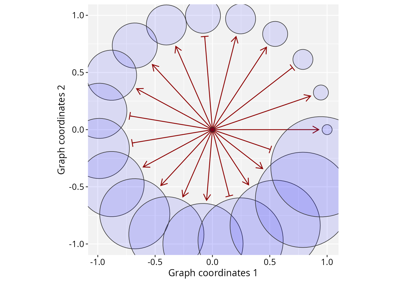

When we map node size to a variable (like the num_var), ggplot2 rescales these values into a target range (e.g., c(2, 40)). This provides all the advantages of the ggplot2 ecosystem, such as flexible graphical scaling and coordinated legends.

There is, however, a subtle trade-off to keep in mind. When node size is mapped via aes(), ggplot2 treats it as a fixed physical dimension (usually in mm) to maintain consistency with the legends. This means the node size will stay locked to the legends and will no longer scale proportionally if the plotting area is resized.

In the example below, geom_graphspace() handles the bulk of the edge adjustment, with the arrow_offset parameter providing additional manual fine-tuning.

ggplot() + 
  geom_graphspace(mapping = aes(size = num_var),
    data = gs_star,  arrow_offset = 0.03) + 
  scale_size(range = c(2, 40)) + 
  theme_gspace_coords() + 
  theme(legend.position = "none")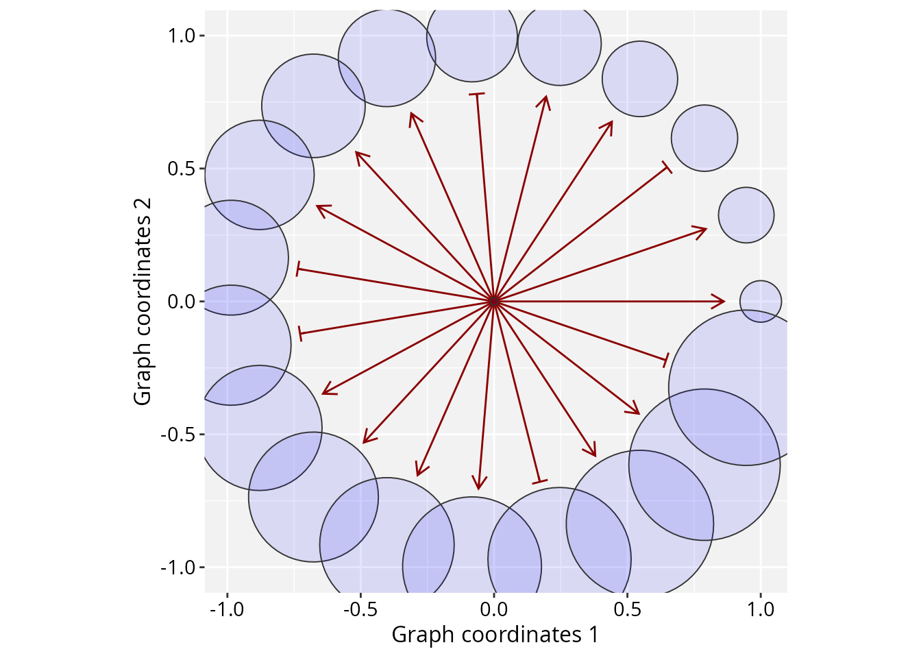

Mapping independent layers

While geom_graphspace() is convenient for quick, coordinated plots, it has a limitation: the mapping argument is reserved for node aesthetics. To overcome this limitation, we can call geom_edgespace() and geom_nodespace() as independent layers. This allows for total flexibility for mapping different variables to edges and nodes.

However, because these layers are now independent, they no longer “talk” to each other by default. If we change the node size scale, the edge layer won’t know it needs to adjust its offsets to accommodate the new node boundaries. To address this, inject_nodespace() acts as a post-processing synchronizer: it intercepts the calculated sizes from the node layer, derive the scaling rules, and “injects” them into the edge layer.

# We shuffle 'num_var' to demonstrate that edges 
# still find their specific boundaries
set.seed(234)
gs_star$num_var2 <- sample(gs_star$num_var)

# Execute the plot, calling 'inject_nodespace' last 
# to capture the final layer states
ggplot(data = gs_star) + 
  geom_edgespace(arrow_offset = 0.03) + 
  geom_nodespace(mapping = aes(size = num_var2 )) + 
  scale_size(range = c(2, 40)) +
  inject_nodespace() +
  theme_gspace_coords() +
  theme(legend.position = "none")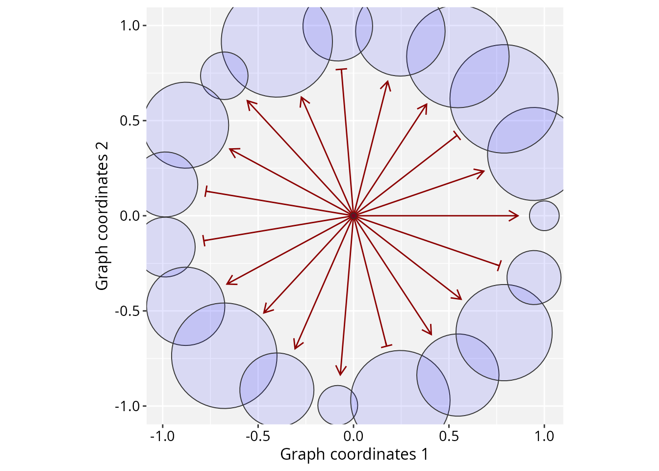

To provide a final note of customization, these scaling trade-offs only apply when size is passed as a node aesthetic mapping. Otherwise, RGraphSpace defaults to using npc units for all network elements.

Session information

#> R version 4.6.0 (2026-04-24)
#> Platform: x86_64-pc-linux-gnu
#> Running under: Ubuntu 24.04.4 LTS
#> 
#> Matrix products: default
#> BLAS:   /usr/lib/x86_64-linux-gnu/openblas-pthread/libblas.so.3 
#> LAPACK: /usr/lib/x86_64-linux-gnu/openblas-pthread/libopenblasp-r0.3.26.so;  LAPACK version 3.12.0
#> 
#> locale:
#>  [1] LC_CTYPE=en_US.UTF-8       LC_NUMERIC=C              
#>  [3] LC_TIME=en_US.UTF-8        LC_COLLATE=en_US.UTF-8    
#>  [5] LC_MONETARY=en_US.UTF-8    LC_MESSAGES=en_US.UTF-8   
#>  [7] LC_PAPER=en_US.UTF-8       LC_NAME=C                 
#>  [9] LC_ADDRESS=C               LC_TELEPHONE=C            
#> [11] LC_MEASUREMENT=en_US.UTF-8 LC_IDENTIFICATION=C       
#> 
#> time zone: America/Sao_Paulo
#> tzcode source: system (glibc)
#> 
#> attached base packages:
#> [1] stats     graphics  grDevices utils     datasets  methods   base     
#> 
#> other attached packages:
#> [1] RGraphSpace_1.3.0 ggplot2_4.0.3     igraph_2.3.1     
#> 
#> loaded via a namespace (and not attached):
#>  [1] gtable_0.3.6       jsonlite_2.0.0     dplyr_1.2.1        compiler_4.6.0    
#>  [5] tidyselect_1.2.1   ggbeeswarm_0.7.3   tidyr_1.3.2        jquerylib_0.1.4   
#>  [9] systemfonts_1.3.2  scales_1.4.0       textshaping_1.0.5  yaml_2.3.12       
#> [13] fastmap_1.2.0      R6_2.6.1           labeling_0.4.3     generics_0.1.4    
#> [17] knitr_1.51         htmlwidgets_1.6.4  tibble_3.3.1       desc_1.4.3        
#> [21] bslib_0.10.0       pillar_1.11.1      RColorBrewer_1.1-3 rlang_1.2.0       
#> [25] cachem_1.1.0       xfun_0.57          fs_2.1.0           sass_0.4.10       
#> [29] S7_0.2.2           otel_0.2.0         cli_3.6.6          withr_3.0.2       
#> [33] pkgdown_2.2.0      magrittr_2.0.5     digest_0.6.39      grid_4.6.0        
#> [37] rstudioapi_0.18.0  beeswarm_0.4.0     lifecycle_1.0.5    vipor_0.4.7       
#> [41] ggrastr_1.0.2      vctrs_0.7.3        evaluate_1.0.5     glue_1.8.1        
#> [45] farver_2.1.2       ragg_1.5.2         tidygraph_1.3.1    purrr_1.2.2       
#> [49] rmarkdown_2.31     tools_4.6.0        pkgconfig_2.0.3    htmltools_0.5.9

Sysbiolab Team

2026-05-23

Overview

Setting basic input data

The problem: static vs. dynamic sizes

Mapping independent layers

Session information