Getting started with RGraphSpace

Package: RGraphSpace 1.4.4

Overview

RGraphSpace is an R package that generates ggplot2 graphics (Wickham 2016) for igraph objects (Csardi and Nepusz 2006) within a normalized coordinate space. This is particularly useful when graph elements must be spatially aligned with reference frames. For comprehensive documentation and use cases, see the online tutorials.

Quick start

To get started, we load a toy igraph and plot it.

#--- Load required packages
library("RGraphSpace")
library("igraph")
library("ggplot2")

# Load the bundled toy igraph object
data("gtoy1", package = "RGraphSpace")

# The most direct call: pass an igraph to plotGraphSpace()
plotGraphSpace(gtoy1, node.labels = TRUE)

Next, we build this toy igraph from scratch to demonstrate the vertex and edge attributes that RGraphSpace parses automatically. This shows exactly what the package expects as input. We use igraph’s make_star() function with V() and E() to assign attributes.

RGraphSpace requires that every vertex carries x, y, and name attributes. If your graph has no pre-existing spatial coordinates, you can supply any igraph layout matrix directly via the layout argument of GraphSpace(), which assigns coordinates internally.

# If your graph has no spatial coordinates, pass a layout directly:
set.seed(42)
GraphSpace(gtoy1, layout = igraph::layout_with_fr(gtoy1))
#> A GraphSpace-class object for:
#> IGRAPH 5fb8aab DN-- 5 4 -- 
#> + attr: x (v/n), y (v/n), name (v/c), nodeLabel (v/c), nodeLabelSize
#> | (v/n), nodeLabelColor (v/c), nodeShape (v/n), nodeSize (v/n),
#> | nodeColor (v/c), nodeLineWidth (v/n), nodeLineColor (v/c), nodeAlpha
#> | (v/n), edgeLineType (e/c), edgeColor (e/c), edgeLineWidth (e/n),
#> | arrowType (e/n), edgeAlpha (e/n)
#> + node spatial boundaries: raw graph
#> | x: [-2, 2] (cols)
#> | y: [-1, 2] (rows)

# Make a 'toy' igraph with 5 nodes and 4 edges;
# ..either a directed or undirected graph
gtoy1 <- make_star(5, mode = "out")

# Check whether the graph is directed or not
is_directed(gtoy1)
#> [1] TRUE

# Check graph size
vcount(gtoy1)
#> [1] 5

ecount(gtoy1)
#> [1] 4

# Assign 'x' and 'y' coordinates to each vertex;
# ..this can be an arbitrary unit in (-Inf, +Inf)
V(gtoy1)$x <- c(0, 2, -2, -4, -8)
V(gtoy1)$y <- c(0, 0,  2, -4,  0)

# Assign a name to each vertex
V(gtoy1)$name <- paste0("n", 1:5)

# Plot the reconstructed 'gtoy1' using RGraphSpace
plotGraphSpace(gtoy1, node.labels = TRUE)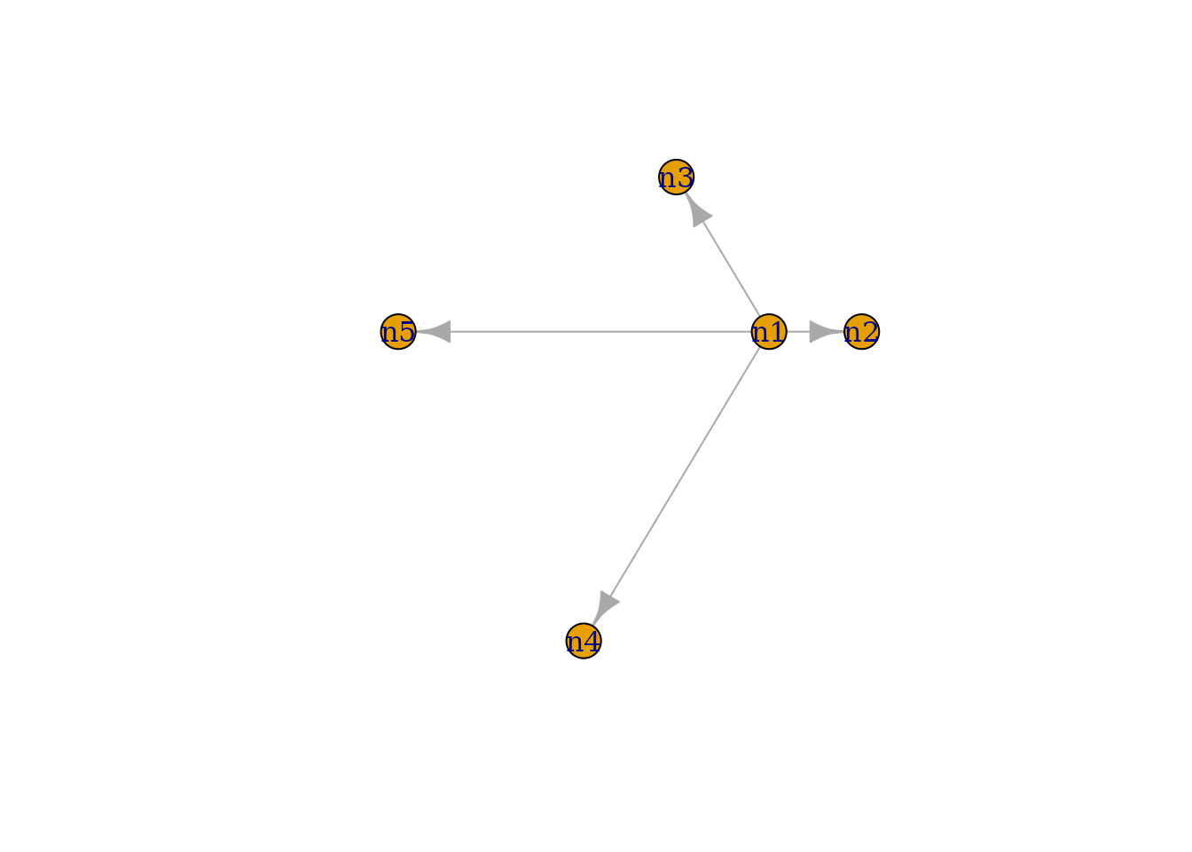

RGraphSpace attributes

Next, we list all vertex and edge attributes that can be passed to RGraphSpace methods.

Vertex attributes

# Node color (Hexadecimal or color name)
V(gtoy1)$nodeColor <- c("red", "#00ad39", "grey80", "lightblue", "cyan")

# Node transparency (in [0,1])
V(gtoy1)$nodeAlpha <- 1

# Node size (numeric in [0, 100], as '%' of the plot space)
V(gtoy1)$nodeSize <- c(8, 5, 5, 10, 5)

# Node shape (integer code between 0 and 25; see 'help(points)')
V(gtoy1)$nodeShape <- c(21, 22, 23, 24, 25)

# Node line width (as in 'lwd' standard graphics; see 'help(gpar)')
V(gtoy1)$nodeLineWidth <- 1

# Node line color (Hexadecimal or color name)
V(gtoy1)$nodeLineColor <- "grey20"

# Node labels ('NA' will omit the label)
V(gtoy1)$nodeLabel <- c("V1", "V2", "V3", "V4", NA)

# Node label size (in mm)
V(gtoy1)$nodeLabelSize <- 3

# Node label color (Hexadecimal or color name)
V(gtoy1)$nodeLabelColor <- "black"

Edge attributes

Given a list of edges, RGraphSpace represents only one edge for each pair of connected vertices. If there are multiple edges connecting the same node pair, it will display the attributes of the first occurrence in the data.

# Edge color (Hexadecimal or color name)
E(gtoy1)$edgeColor <- c("red","green","blue","black")

# Edge transparency (in [0,1])
E(gtoy1)$edgeAlpha <- 1

# Edge line width (as in 'lwd' standard graphics; see 'help(gpar)')
E(gtoy1)$edgeLineWidth <- 0.8

# Edge line type (as in 'lty' standard graphics; see 'help(gpar)')
E(gtoy1)$edgeLineType <- c("solid", "11", "dashed", "2124")

Note: edgeLineColor is deprecated as of version 1.4.3 and replaced by edgeColor.

Arrowhead attributes

Arrowhead in directed graphs: By default, an arrow will be drawn for each edge according to its left-to-right orientation in the edge list (e.g. A -> B). If there are mutual connections, the package will recode the mutual edges to represent a bidirectional flow.

# Arrowhead types in directed graphs
## Integer or character code:
## 0 = "---", 1 = "-->", -1 = "--|"
E(gtoy1)$arrowType <- 1

Arrowhead in undirected graphs: By default, no arrow will be drawn for undirected graphs. However, arrowheads may be assigned according to the coding below.

# Arrowhead types in undirected graphs
## Integer or character code:
##  0 = "---"
##  1 = "-->",  2 = "<--",  3 = "<->",  4 = "|->"
## -1 = "--|", -2 = "|--", -3 = "|-|", -4 = "<-|"
gtoy1_undir <- igraph::as_undirected(gtoy1, edge.attr.comb = "first")
E(gtoy1_undir)$arrowType <- 1
# Note: in undirected graphs, this attribute overrides
# the edge's orientation in the edge list and adds arrowheads
# to edges that would otherwise be drawn without any

… and plot the fully attributed gtoy1 object.

# Plot the fully attributed 'gtoy1'
plotGraphSpace(gtoy1, node.labels = TRUE)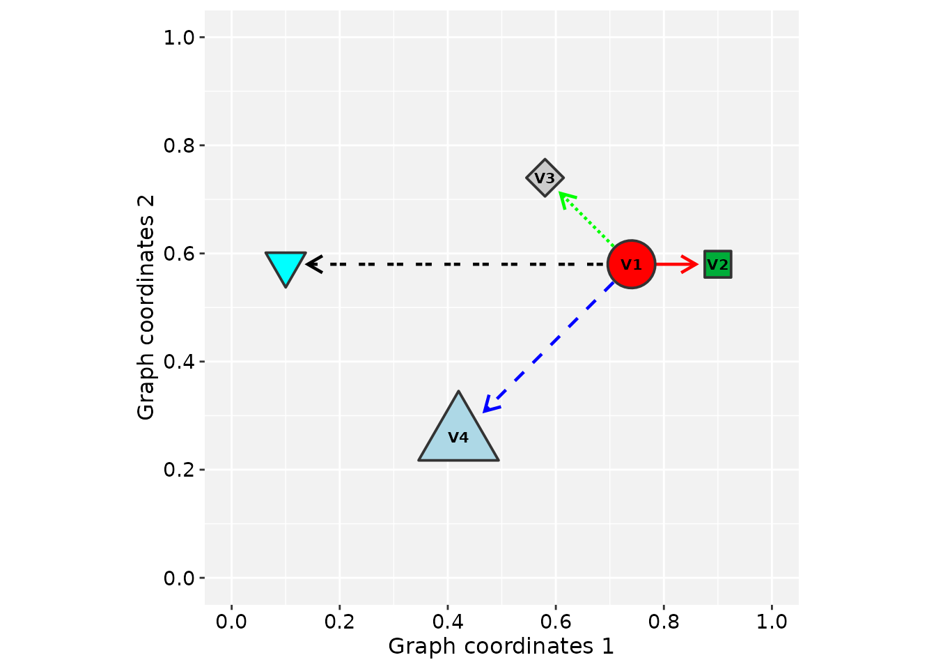

Passing graphs to geoms

Alternatively, an igraph can be converted to a GraphSpace object and passed directly to ggplot2 geoms. This gives full access to the ggplot2 layer system for combining graph elements with other plot types.

# Load the toy graph used in the previous example
data("gtoy1", package = "RGraphSpace")

# Create a GraphSpace object
gs <- GraphSpace(gtoy1)
#> Validating the 'igraph' object...
#> Ignoring graph-level attributes: 'name', 'mode', 'center'
#> Creating a 'GraphSpace' object...

# Normalize the coordinates
gs <- normalizeGraphSpace(gs)
#> Normalizing node coordinates to graph space...

gs
#> A GraphSpace-class object for:
#> IGRAPH 5fb8aab DN-- 5 4 -- 
#> + attr: x (v/n), y (v/n), name (v/c), nodeLabel (v/c), nodeLabelSize
#> | (v/n), nodeLabelColor (v/c), nodeShape (v/n), nodeSize (v/n),
#> | nodeColor (v/c), nodeLineWidth (v/n), nodeLineColor (v/c), nodeAlpha
#> | (v/n), edgeLineType (e/c), edgeColor (e/c), edgeLineWidth (e/n),
#> | arrowType (e/n), edgeAlpha (e/n)
#> + node spatial boundaries: normalized to graph space
#> | x: [-8, 2] -> [0, 1] (cols)
#> | y: [-4, 2] -> [0, 1] (rows)

normalizeGraphSpace() maps all vertex coordinates to a [0, 1] unit interval and computes the per-node clipping offsets that allow geom_edgespace() to terminate edges precisely at node boundaries. This step is handled automatically when you use plotGraphSpace(), but must be called explicitly when building a plot layer by layer.

# Build a layered ggplot2 graph
# geom_edgespace() draws edges; geom_nodespace() draws nodes
# aes(label = nodeLabel) maps the 'nodeLabel' vertex attribute to node labels
ggplot(gs) + 
  geom_edgespace() + 
  geom_nodespace(aes(label = nodeLabel)) + 
  theme_gspace_coords(is_norm = TRUE)

Online tutorials

For detailed integration with the ggplot2 ecosystem, see the online documentation available at:

https://sysbiolab.github.io/RGraphSpace/

Other examples

Vignettes illustrating how RGraphSpace can be used in combination with PathwaySpace to project network signals.

https://sysbiolab.github.io/PathwaySpace/

Citation

If you use RGraphSpace, please cite:

Sysbiolab Team. “RGraphSpace: A lightweight interface between igraph and ggplot2 graphics.” R package, 2023. Doi: 10.32614/CRAN.package.RGraphSpace

Session information

#> R version 4.6.1 (2026-06-24)
#> Platform: x86_64-pc-linux-gnu
#> Running under: Ubuntu 24.04.4 LTS
#> 
#> Matrix products: default
#> BLAS:   /usr/lib/x86_64-linux-gnu/openblas-pthread/libblas.so.3 
#> LAPACK: /usr/lib/x86_64-linux-gnu/openblas-pthread/libopenblasp-r0.3.26.so;  LAPACK version 3.12.0
#> 
#> locale:
#>  [1] LC_CTYPE=en_US.UTF-8       LC_NUMERIC=C              
#>  [3] LC_TIME=en_US.UTF-8        LC_COLLATE=en_US.UTF-8    
#>  [5] LC_MONETARY=en_US.UTF-8    LC_MESSAGES=en_US.UTF-8   
#>  [7] LC_PAPER=en_US.UTF-8       LC_NAME=C                 
#>  [9] LC_ADDRESS=C               LC_TELEPHONE=C            
#> [11] LC_MEASUREMENT=en_US.UTF-8 LC_IDENTIFICATION=C       
#> 
#> time zone: America/Sao_Paulo
#> tzcode source: system (glibc)
#> 
#> attached base packages:
#> [1] stats     graphics  grDevices utils     datasets  methods   base     
#> 
#> other attached packages:
#> [1] igraph_2.3.3      RGraphSpace_1.4.4 ggplot2_4.0.3    
#> 
#> loaded via a namespace (and not attached):
#>  [1] Matrix_1.7-5       gtable_0.3.6       jsonlite_2.0.0     dplyr_1.2.1       
#>  [5] compiler_4.6.1     tidyselect_1.2.1   ggbeeswarm_0.7.3   tidyr_1.3.2       
#>  [9] jquerylib_0.1.4    systemfonts_1.3.2  scales_1.4.0       textshaping_1.0.5 
#> [13] yaml_2.3.12        fastmap_1.2.0      lattice_0.22-9     R6_2.6.1          
#> [17] generics_0.1.4     knitr_1.51         htmlwidgets_1.6.4  tibble_3.3.1      
#> [21] desc_1.4.3         bslib_0.11.0       pillar_1.11.1      RColorBrewer_1.1-3
#> [25] rlang_1.2.0        cachem_1.1.0       xfun_0.59          fs_2.1.0          
#> [29] sass_0.4.10        S7_0.2.2           otel_0.2.0         cli_3.6.6         
#> [33] pkgdown_2.2.0      withr_3.0.3        magrittr_2.0.5     digest_0.6.39     
#> [37] grid_4.6.1         rstudioapi_0.19.0  beeswarm_0.4.0     lifecycle_1.0.5   
#> [41] vipor_0.4.7        ggrastr_1.0.2      vctrs_0.7.3        evaluate_1.0.5    
#> [45] glue_1.8.1         farver_2.1.2       ragg_1.5.2         tidygraph_1.3.1   
#> [49] purrr_1.2.2        rmarkdown_2.31     tools_4.6.1        pkgconfig_2.0.3   
#> [53] htmltools_0.5.9

References

Csardi, Gabor, and Tamas Nepusz. 2006. “The Igraph Software Package for Complex Network Research.” InterJournal Complex Systems: 1695. https://igraph.org/.

Wickham, Hadley. 2016. Ggplot2: Elegant Graphics for Data Analysis. Springer-Verlag New York. https://ggplot2.tidyverse.org.

Sysbiolab Team

2026-07-21