Visualizing spatial transcriptomics
Gene expression projections on spot coordinates
Sysbiolab Team
2026-06-23
Source:vignettes/articles/spatial-transcriptomics.Rmd
spatial-transcriptomics.RmdPackage: PathwaySpace 1.4.1
Overview
This vignette introduces PathwaySpace as an extension for the Seurat package (Hao et al. 2024), providing methods for signal projection and visualization in spatial transcriptomics. It extends existing spatial analysis workflows to explore signal patterns in tissue microenvironments. In what follows, we present three step-by-step tutorials describing how to prepare input data for PathwaySpace. The results reproduce and refine examples featured in Seurat’s tutorials, so users are encouraged to see how these packages can be used together.
Before you start
This vignette assumes prior experience with Seurat (Hao et al. 2024), especially for handling spatial transcriptomics data.
Note: If you are new to Seurat’s spatial workflows, we recommend reviewing the spatial analysis tutorials before continuing.
Computational requirement:
Hardware: RAM >= 16 GB
Software: R (>=4.5) and RStudio
Required packages
Ensure that all packages described in the Installation Instructions are installed.
# Check required versions
if (packageVersion("RGraphSpace") < "1.4.1"){
  message("Need to update 'RGraphSpace' for this vignette")
  remotes::install_github("sysbiolab/RGraphSpace")
}
if (packageVersion("PathwaySpace") < "1.4.1"){
  message("Need to update 'PathwaySpace' for this vignette")
  remotes::install_github("sysbiolab/PathwaySpace")
}
if (packageVersion("Seurat") < "5.5.0"){
  message("Need to update 'Seurat' for this vignette")
  remotes::install_github("satijalab/Seurat")
}
# Load packages
library("RGraphSpace")
library("PathwaySpace")
library("Seurat")
library("SeuratObject")
library("SeuratData")
library("patchwork")
Visium v1 dataset
Setting input data
For this tutorial, we will use the stxBrain dataset from
the SeuratData package, consisting of spatial transcriptomics
data from sagittal mouse brain sections generated with Visium v1
technology. This dataset is commonly used to demonstrate Seurat
spatial workflows (Hao et al. 2024). Here,
we will preprocess it with Seurat and then extract the relevant
data for PathwaySpace downstream analyses.
## Install a Seurat dataset (this step is required only once)
SeuratData::InstallData("stxBrain")
# Check manifest of installed datasets
# SeuratData::InstalledData()

# Load the 'stxBrain' dataset
# Note: LoadData() may print conversion warnings when loading pbmc3k.
# These are expected and come from SeuratData's internal v4-to-v5
# object migration — they can be safely ignored.
seurat_obj <- LoadData("stxBrain", type = "anterior1")
The stxBrain dataset is preprocessed following
Seurat’s spatial analysis workflow, including
variance-stabilizing normalization and cluster annotation.
# Normalize, reduce dimensions, and annotate clusters
seurat_obj <- SCTransform(seurat_obj, assay = "Spatial", verbose = FALSE)
seurat_obj <- RunPCA(seurat_obj, assay = "SCT", verbose = FALSE)
seurat_obj <- FindNeighbors(seurat_obj, reduction = "pca", dims = 1:30)
seurat_obj <- FindClusters(seurat_obj, verbose = FALSE)
… and then as.GraphSpace() converts the Seurat
object into a GraphSpace, exposing its spatial coordinates
and feature data to the ggplot2 grammar. We then attach the
tissue image and normalize node coordinates to the image space.
# Create a GraphSpace from 'seurat_obj'
gs <- as.GraphSpace(seurat_obj, space = "spatial", scale = "lowres")

# Seurat object converted to GraphSpace:
# ℹ space=spatial, layer=default, features=17668, samples=2696, scale="lowres"
# Node spatial boundaries:
# ℹ x: [76, 493] (cols)
# ℹ y: [138, 541] (rows)
# If available, add tissue image
gs_image(gs) <- SeuratObject::GetImage(seurat_obj, mode = "raster")

# Image spatial boundaries:
# ℹ x: [1, 600] (cols)
# ℹ y: [1, 599] (rows)
# Normalize node coordinates to the image space
# By default, this attempts to align the graph's bottom-up
# coordinates with the image's top-down matrix layout.
gs <- normalizeGraphSpace(gs)

# Inspect the 'gs' object
gs
# A GraphSpace-class object for:
# IGRAPH 381ac9a UN-- 2696 0 --
# + attr: x (v/n), y (v/n), name (v/c), nodeLabel (v/c), nodeSize
# | (v/n), cell (v/c), orig.ident (v/x), nCount_Spatial (v/n),
# | nFeature_Spatial (v/n), slice (v/n), region (v/c), nCount_SCT
# | (v/n), nFeature_SCT (v/n), SCT_snn_res.0.8 (v/x), seurat_clusters
# | (v/x), arrowType (e/n)
# + features: 17668 (Xkr4, Sox17, Mrpl15, Lypla1, ...)
In this tutorial we use the low-level ggplot2 interface for
fine-grained control; the subsequent tutorials use the higher-level
plotPathwaySpace() wrapper for convenience.
# Set a reusable theme for spatial plots
spatial_theme <- theme_gspace_coords(theme = "th3", is_norm = TRUE,
  xlab = "Spot coordinates 1", ylab = "Spot coordinates 2")

# Left: 'seurat_clusters' annotation overlaid on tissue image
cpal1 <- DiscretePalette(nlevels(gs$seurat_clusters), "polychrome")
p1 <- ggplot(gs) +
  annotation_gspace_image(gs, opacity = 0.5) +
  geom_nodespace(mapping = aes(colour = seurat_clusters), size=0.8, pch=19) +
  scale_colour_discrete(palette = cpal1) +
  theme_gspace_legend(discrete_colour = TRUE) +
  spatial_theme

# Right: Camk2n1 gene expression overlaid on tissue image
cpal2 <- hcl.colors(100, palette = "Spectral", rev = TRUE)
p2 <- ggplot(gs) +
  annotation_gspace_image(gs, opacity = 0.5) +
  geom_nodespace(mapping = aes(colour = Camk2n1), size=0.8, pch=19) +
  scale_colour_continuous(palette = cpal2) +
  spatial_theme

p1 + p2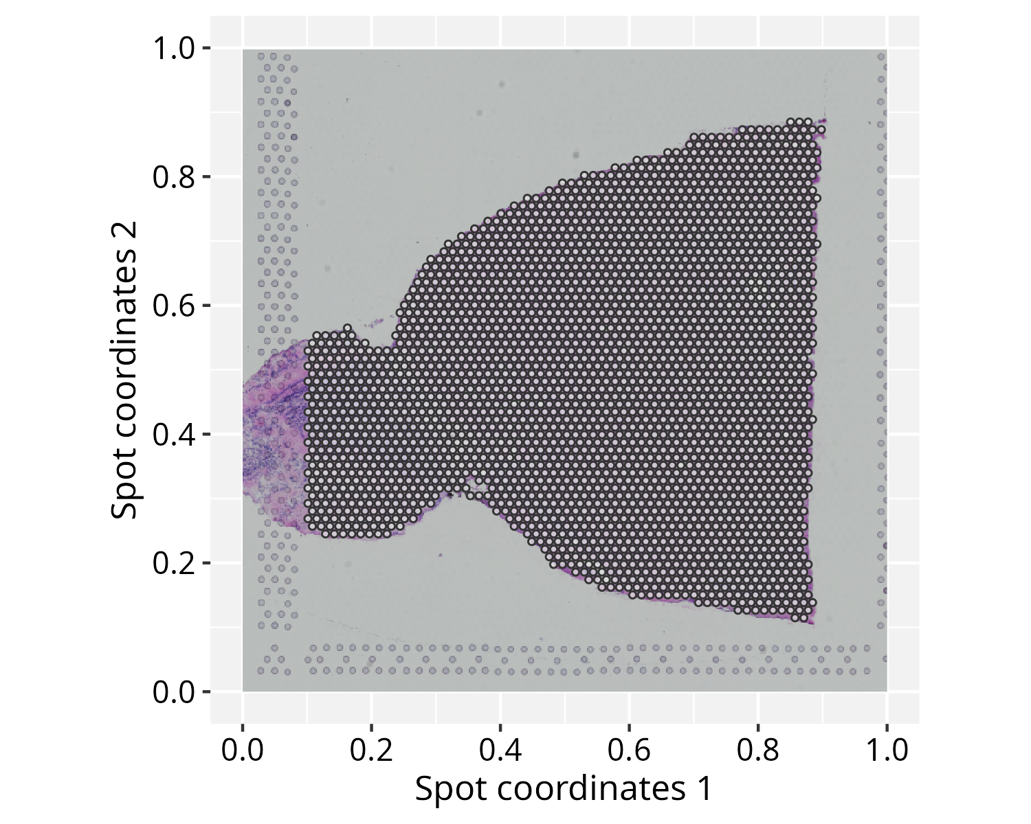
Note on image alignment: Proper spatial alignment
between spot coordinates and the background image requires consistent
coordinate conventions. Spatial misalignment may occur when the input
spot coordinates and image follow origin placements or axis orientations
that differ from the package’s internal coordinate definitions (e.g.,
top-left versus bottom-left origins). To accommodate these differences,
normalizeGraphSpace() provides orientation controls through
the flip.* and rotate.* arguments. If the
spots appear misaligned with the input image, try alternative
combinations of these parameters to correct the alignment.
Running PathwaySpace
# Create a PathwaySpace object
pspace_obj <- buildPathwaySpace(gs)
Before running the projection, we need to specify a distance unit for the signal decay function. This unit will affect the extent over which the signal is projected on the coordinate space. We will use the center-to-center distance between spots, corresponding to 100 µm in Visium v1 technology.
# Get distance to the nearest spot
nspot <- getNearestNode(pspace_obj)
pdist <- mean(nspot$dist) # average distance
# 'pdist' is set as the average center-to-center distance between spots
pdist
# [1] 0.013
As an optional step, the silhouetteMapping() function
generates an image mask that outlines the graph layout, over which the
subsequent methods will project a landscape image. The
baseline argument controls the level at which a silhouette
is sliced to form the mask. Increasing the baseline (in
[0,1]) produces a more detailed, granular silhouette.
# Add a graph silhouette to the PathwaySpace object
pspace_obj <- silhouetteMapping(pspace_obj, baseline = 0.1)

# Check the silhouette plot
ggplot(pspace_obj) +
  annotation_gspace_image(pspace_obj) +
  annotation_pspace_signal(pspace_obj, si.alpha = 0.5) +
  spatial_theme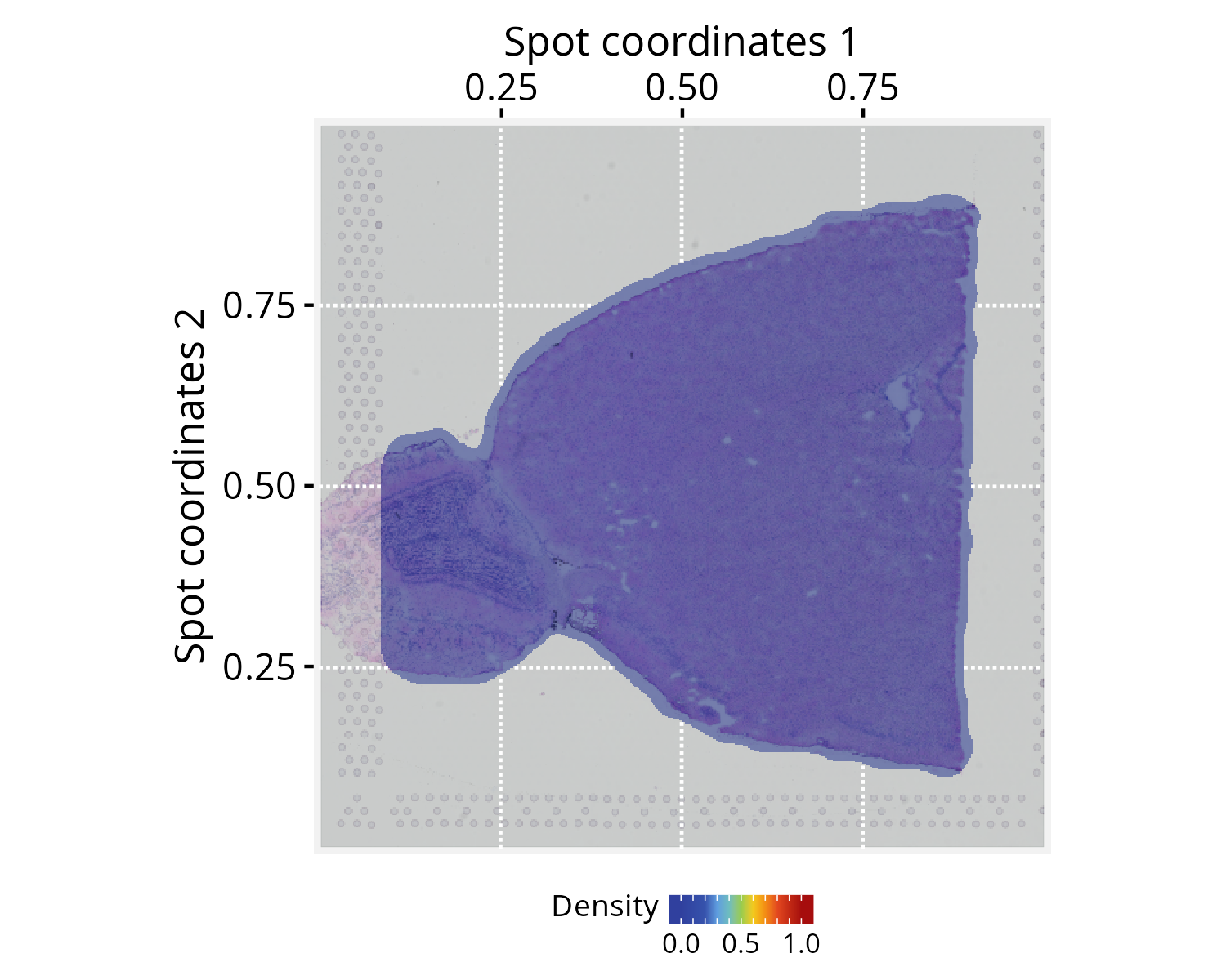
Next, we specify the signal to be projected. Here we use expression
data from the Camk2n1 gene, set via the
activeFeature() accessor, which automatically loads the
corresponding signal into the projection pipeline.
# Set a 'feature' of interest for signal
# projection (e.g., Camk2n1 gene)
activeFeature(pspace_obj) <- "Camk2n1"
We then perform the signal projection, setting
decay = 0.5. The decay parameter controls how the signal
attenuates with distance; at decay = 0.5, the signal
decreases to half of its initial value at a distance equal to
pdist (for additional configuration details, see the modeling signal decay
tutorial).
# Project gene signal
pspace_obj <- circularProjection(pspace_obj,
  k = gs_vcount(pspace_obj),
  decay.fun = weibullDecay(decay=0.5, pdist = pdist),
  aggregate.fun = signalAggregation("wmean"))
Because each spot produces an independent projection, the resulting
projections are aggregated into a unified landscape. Here we use a
weighted arithmetic mean, where each projection is weighted by its own
magnitude (for additional details, see the signal aggregation
rules tutorial). The k parameter controls the
aggregation by determining how many projected signals are considered at
each point in space. The default k = gs_vcount(ps) retains
contributions from all vertices.
Next, we demonstrate the plotting interface with a few variations to highlight key settings.
# Left: tissue image only, no signal overlay
p1 <- ggplot(pspace_obj) +
  annotation_gspace_image(pspace_obj) +
  spatial_theme

# Right: signal overlaid on tissue image with low opacity
p2 <- ggplot(pspace_obj) +
  annotation_gspace_image(pspace_obj) +
  annotation_pspace_signal(pspace_obj, si.alpha = 0.5) +
  spatial_theme

p1 + p2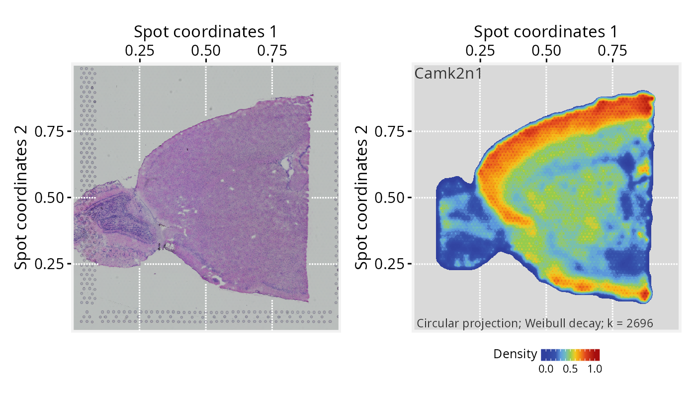
# Left: signal overlaid on tissue image with low opacity
p2 <- ggplot(pspace_obj) +
  annotation_gspace_image(pspace_obj) +
  annotation_pspace_signal(pspace_obj, si.alpha = 0.25) +
  spatial_theme

# Right: same, with signal truncated to the upper range (zlim >= 0.5)
p3 <- ggplot(pspace_obj) +
  annotation_gspace_image(pspace_obj) +
  annotation_pspace_signal(pspace_obj, si.alpha = 0.25, zlim = c(0.5, 1)) +
  spatial_theme

p2 + p3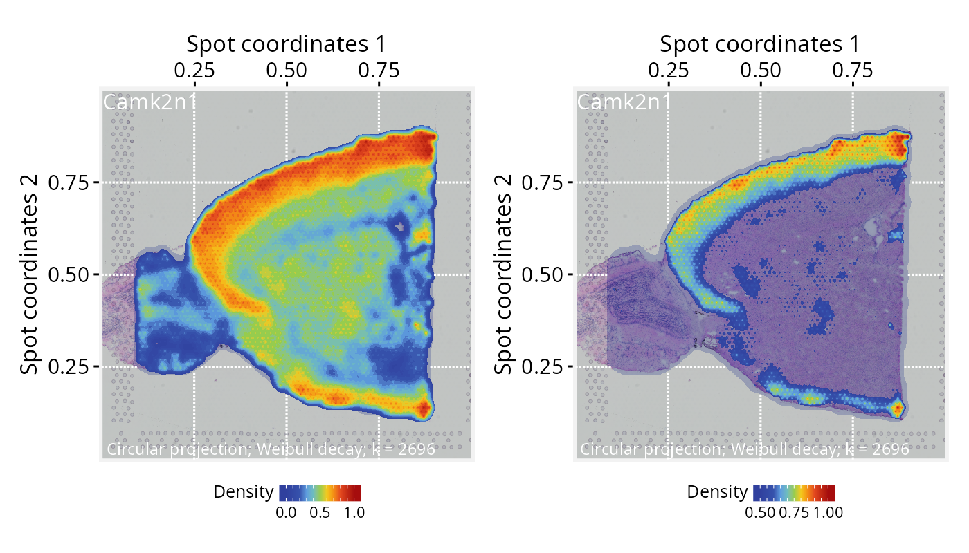
Slide-seq v2 dataset
Setting input data
For this tutorial, we will use the ssHippo dataset
available from the SeuratData package, consisting of spatial
transcriptomics data from mouse hippocampus generated with
Slide-seq v2 technology. We will follow the same
general steps from our previous spatial tutorial, preprocessing with
Seurat and then extracting the relevant data for
PathwaySpace downstream analyses. For further details on this
dataset, see Seurat’s spatial_vignette.
## Install a Seurat dataset (this step is required only once)
SeuratData::InstallData("ssHippo")
# Check manifest of installed datasets
# SeuratData::InstalledData()

# Load the 'kidneyref' dataset
seurat_obj <- LoadData("ssHippo")
# Run vst normalization on counts
# seurat_obj <- SCTransform(seurat_obj, assay = "Spatial", verbose = FALSE)

# NOTE: Seurat recommends using SCTransform() for processing this
# spatial dataset, which may require more computation time. Here,
# we use log-normalization for demonstration purposes.
seurat_obj <- NormalizeData(seurat_obj)
seurat_obj
# An object of class Seurat
# 23264 features across 53173 samples within 1 assay
# Active assay: Spatial (23264 features, 0 variable features)
#  2 layers present: counts, data
#  1 image present: image
# Create a GraphSpace from 'seurat_obj'
gs <- as.GraphSpace(seurat_obj, space = "spatial", layer = "data")

#Note: the `ssHippo` dataset does not include a tissue image

# Normalize node coordinates; adjust 'flip.y' and 'rotate.xy' to
# follow image orientation in Seurat's vignette
gs <- normalizeGraphSpace(gs, flip.y = TRUE, rotate.xy = TRUE)

# If needed, remove seurat_obj to free memory
# rm(seurat_obj)
Running PathwaySpace
# Create a PathwaySpace from the 'gs' object
pspace_obj <- buildPathwaySpace(gs)
# Get distance to the nearest spot
nspot <- getNearestNode(pspace_obj)
pdist <- mean(nspot$dist) # average distance
# 'pdist' set as the average center-to-center distance between spots
pdist
# [1] 0.0024
# Add a graph silhouette to the PathwaySpace object
pspace_obj <- silhouetteMapping(pspace_obj, fill.cavity = FALSE,
  pdist = max(nspot$dist))

# Check silhouette plot
plotPathwaySpace(ps=pspace_obj, theme = "th3", si.alpha = 0.5)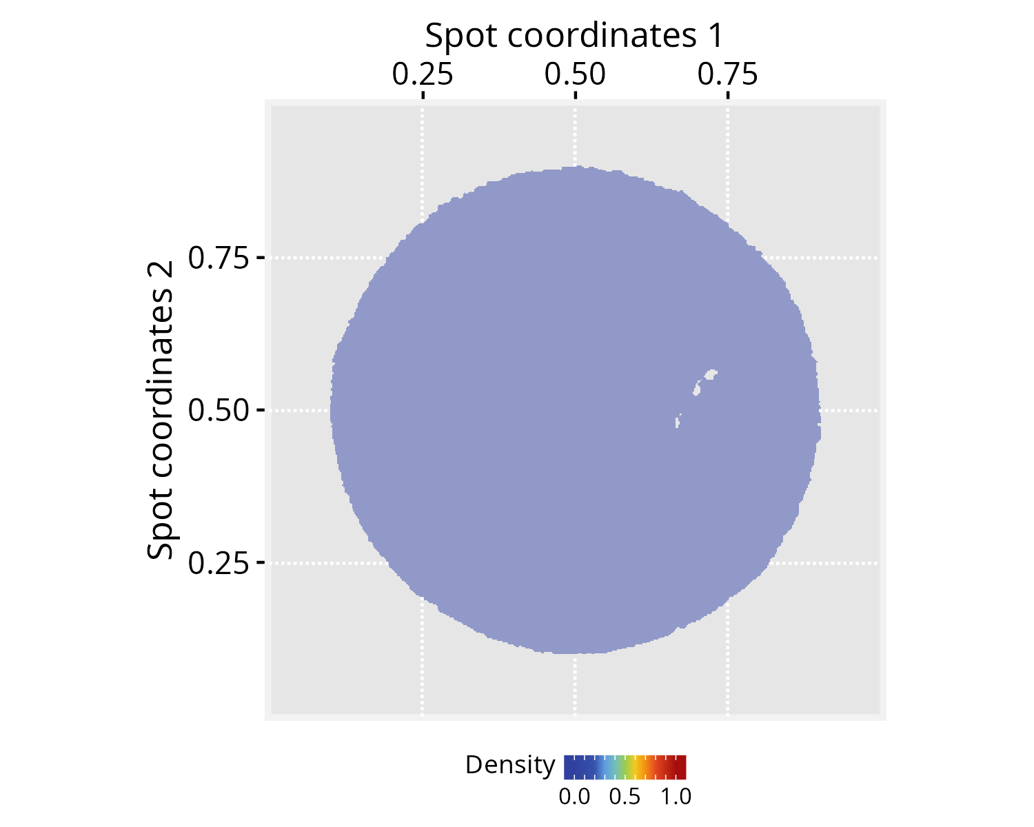
# Set a 'feature' of interest for signal
# projection (e.g., DDN gene)
activeFeature(pspace_obj) <- "DDN"

# Project gene signal
pspace_obj <- circularProjection(pspace_obj,
  k = gs_vcount(pspace_obj),
  decay.fun = weibullDecay(decay=0.5, pdist = pdist))

# Plot projections
p1 <- plotPathwaySpace(ps = pspace_obj, theme = "th3")
# ...another 'feature' (e.g. PCP4 gene)
activeFeature(pspace_obj) <- "PCP4"

# Project gene signal
pspace_obj <- circularProjection(pspace_obj, k = gs_vcount(pspace_obj),
  decay.fun = weibullDecay(decay=0.5, pdist = pdist))

# Plot projections
p2 <- plotPathwaySpace(ps = pspace_obj, theme = "th3")
p1 + p2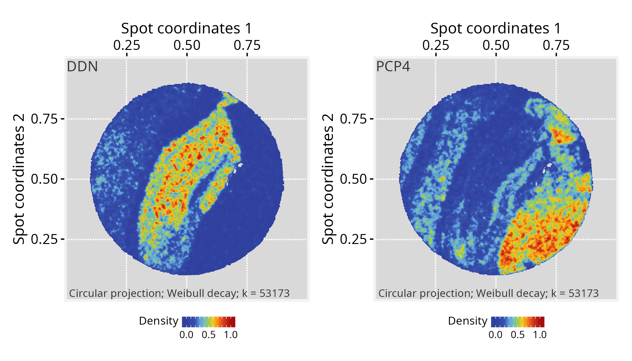
Visium HD dataset
Setting input data
Here, we will use a higher-resolution spatial dataset from mouse brain generated with Visium HD technology. This platform provides whole-transcriptome gene expression data at a raw 2-µm resolution, with additional binned versions available at 8 and 16 µm. For this tutorial, we will use the 16-µm binned data. We will follow the same general steps from our previous spatial tutorials, preprocessing with Seurat and then extracting the relevant data for PathwaySpace downstream analyses. For additional details on this dataset, refer to Seurat’s visiumhd_analysis_vignette.
The Visium HD dataset can be downloaded from the 10x Genomics repository:
- Repository URL: https://www.10xgenomics.com/datasets
- Dataset: Visium HD Spatial Gene Expression Library, Mouse Brain (FFPE)
- Where to find it: Output and supplemental files
- Download: Binned outputs (all bin levels)
- File: Visium_HD_Mouse_Brain_binned_outputs.tar.gz
- MD5: 2e728d1c1bda99a36535ba45b4319a98
- Size: 4.62 GB
# Extract the tar.gz and set 'localdir' to the dataset folder
# Use 'bin.size' to choose the data resolution to load (2, 8, or 16 µm)
localdir <- "path/to/data/directory"
seurat_obj <- Load10X_Spatial(data.dir = localdir, bin.size = 16)

# Check default assay
Assays(seurat_obj)
# [1] "Spatial.016um"
# Run log-normalization for spatial data
seurat_obj <- NormalizeData(seurat_obj)
# Create a GraphSpace from 'seurat_obj'
gs <- as.GraphSpace(seurat_obj, space = "spatial", scale = "lowres")

# If available, add tissue image
gs_image(gs) <- SeuratObject::GetImage(seurat_obj, mode = "raster")

# Normalize node coordinates to the image space
gs <- normalizeGraphSpace(gs)

# If needed, remove seurat_obj to free memory
rm(seurat_obj)
# Create a PathwaySpace object from 'gs' mapped to the 'raster'
pspace_obj <- buildPathwaySpace(gs, nrc = 700)
Running PathwaySpace
# Get distance to the nearest spot
nspot <- getNearestNode(pspace_obj)
pdist <- mean(nspot$dist) # average distance
# 'pdist' set as the average center-to-center distance between spots
pdist
# [1] 0.0024
# Add a graph silhouette to the PathwaySpace object
pspace_obj <- silhouetteMapping(pspace_obj,
  fill.cavity = FALSE,
  pdist = max(nspot$dist))

# Check silhouette plot
plotPathwaySpace(ps = pspace_obj, theme = "th3",
  add.image = TRUE, si.alpha = 0.5)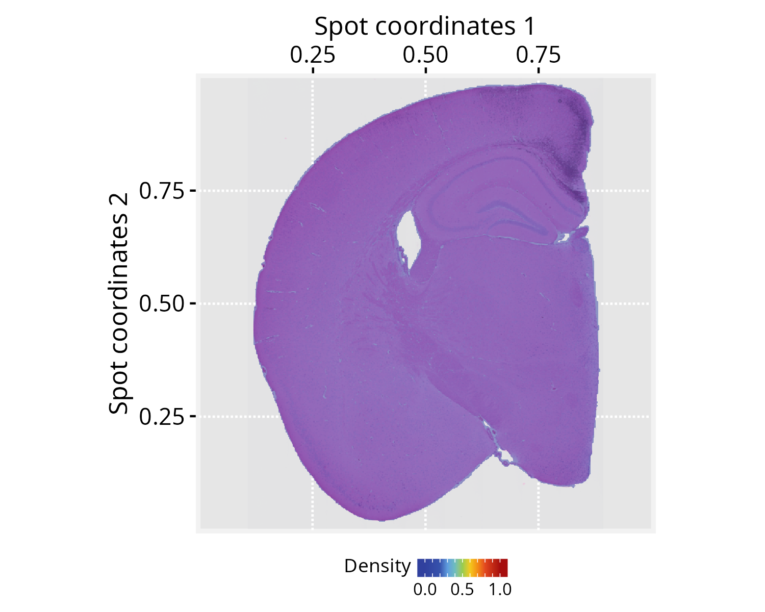
# Set a 'feature' of interest for signal
# projection (e.g., Rorb gene)
activeFeature(pspace_obj) <- "Rorb"

# Project gene signal
pspace_obj <- circularProjection(pspace_obj, k = gs_vcount(pspace_obj),
  decay.fun = weibullDecay(decay=0.5, pdist = pdist))

# Plot projections
p1 <- plotPathwaySpace(pspace_obj, theme = "th3", add.image = TRUE)
# ...another 'feature' (e.g. Hpca gene)
activeFeature(pspace_obj) <- "Hpca"

# Project gene signal
pspace_obj <- circularProjection(pspace_obj, k = gs_vcount(pspace_obj),
  decay.fun = weibullDecay(decay=0.5, pdist = pdist))

# Plot projections
p2 <- plotPathwaySpace(pspace_obj, theme = "th3", add.image = TRUE)
p1 + p2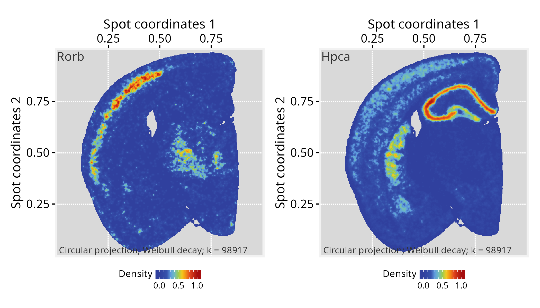
Citation
If you use PathwaySpace, please cite:
Tercan & Apolonio et al. Protocol for assessing distances in pathway space for classifier feature sets from machine learning methods. STAR Protocols 6(2):103681, 2025. https://doi.org/10.1016/j.xpro.2025.103681
Ellrott et al. Classification of non-TCGA cancer samples to TCGA molecular subtypes using compact feature sets. Cancer Cell 43(2):195-212.e11, 2025. https://doi.org/10.1016/j.ccell.2024.12.002
Session information
#> R version 4.6.0 (2026-04-24)
#> Platform: x86_64-pc-linux-gnu
#> Running under: Ubuntu 24.04.4 LTS
#>
#> Matrix products: default
#> BLAS:   /usr/lib/x86_64-linux-gnu/openblas-pthread/libblas.so.3
#> LAPACK: /usr/lib/x86_64-linux-gnu/openblas-pthread/libopenblasp-r0.3.26.so;  LAPACK version 3.12.0
#>
#> locale:
#>  [1] LC_CTYPE=en_US.UTF-8       LC_NUMERIC=C
#>  [3] LC_TIME=en_US.UTF-8        LC_COLLATE=en_US.UTF-8
#>  [5] LC_MONETARY=en_US.UTF-8    LC_MESSAGES=en_US.UTF-8
#>  [7] LC_PAPER=en_US.UTF-8       LC_NAME=C
#>  [9] LC_ADDRESS=C               LC_TELEPHONE=C
#> [11] LC_MEASUREMENT=en_US.UTF-8 LC_IDENTIFICATION=C
#>
#> time zone: America/Sao_Paulo
#> tzcode source: system (glibc)
#>
#> attached base packages:
#> [1] stats     graphics  grDevices utils     datasets  methods   base
#>
#> other attached packages:
#>  [1] patchwork_1.3.2           stxBrain.SeuratData_0.1.2
#>  [3] ssHippo.SeuratData_3.1.4  pbmc3k.SeuratData_3.1.4
#>  [5] SeuratData_0.2.2.9002     Seurat_5.5.0
#>  [7] SeuratObject_5.4.0        sp_2.2-1
#>  [9] PathwaySpace_1.4.1        RGraphSpace_1.4.1
#> [11] ggplot2_4.0.3
#>
#> loaded via a namespace (and not attached):
#>   [1] RColorBrewer_1.1-3     rstudioapi_0.18.0      jsonlite_2.0.0
#>   [4] magrittr_2.0.5         spatstat.utils_3.2-3   ggbeeswarm_0.7.3
#>   [7] farver_2.1.2           rmarkdown_2.31         fs_2.1.0
#>  [10] ragg_1.5.2             vctrs_0.7.3            ROCR_1.0-12
#>  [13] spatstat.explore_3.8-1 htmltools_0.5.9        sass_0.4.10
#>  [16] sctransform_0.4.3      parallelly_1.47.0      KernSmooth_2.23-26
#>  [19] bslib_0.11.0           htmlwidgets_1.6.4      desc_1.4.3
#>  [22] ica_1.0-3              fontawesome_0.5.3      plyr_1.8.9
#>  [25] plotly_4.12.0          zoo_1.8-15             cachem_1.1.0
#>  [28] igraph_2.3.2           mime_0.13              lifecycle_1.0.5
#>  [31] pkgconfig_2.0.3        Matrix_1.7-5           R6_2.6.1
#>  [34] fastmap_1.2.0          fitdistrplus_1.2-6     future_1.70.0
#>  [37] shiny_1.13.0           digest_0.6.39          colorspace_2.1-2
#>  [40] ggnewscale_0.5.2       tensor_1.5.1           RSpectra_0.16-2
#>  [43] irlba_2.3.7            textshaping_1.0.5      progressr_0.19.0
#>  [46] spatstat.sparse_3.2-0  httr_1.4.8             polyclip_1.10-7
#>  [49] abind_1.4-8            compiler_4.6.0         withr_3.0.2
#>  [52] S7_0.2.2               fastDummies_1.7.6      MASS_7.3-65
#>  [55] rappdirs_0.3.4         tools_4.6.0            vipor_0.4.7
#>  [58] lmtest_0.9-40          otel_0.2.0             beeswarm_0.4.0
#>  [61] httpuv_1.6.17          future.apply_1.20.2    goftest_1.2-3
#>  [64] glue_1.8.1             nlme_3.1-169           promises_1.5.0
#>  [67] grid_4.6.0             Rtsne_0.17             cluster_2.1.8.2
#>  [70] reshape2_1.4.5         generics_0.1.4         gtable_0.3.6
#>  [73] spatstat.data_3.1-9    tidyr_1.3.2            data.table_1.18.4
#>  [76] tidygraph_1.3.1        spatstat.geom_3.8-1    RcppAnnoy_0.0.23
#>  [79] ggrepel_0.9.8          RANN_2.6.2             pillar_1.11.1
#>  [82] stringr_1.6.0          spam_2.11-4            RcppHNSW_0.7.0
#>  [85] later_1.4.8            splines_4.6.0          dplyr_1.2.1
#>  [88] lattice_0.22-9         survival_3.8-6         deldir_2.0-4
#>  [91] tidyselect_1.2.1       miniUI_0.1.2           pbapply_1.7-4
#>  [94] knitr_1.51             gridExtra_2.3          scattermore_1.2
#>  [97] xfun_0.58              matrixStats_1.5.0      stringi_1.8.7
#> [100] lazyeval_0.2.3         yaml_2.3.12            evaluate_1.0.5
#> [103] codetools_0.2-20       tibble_3.3.1           cli_3.6.6
#> [106] uwot_0.2.4             xtable_1.8-8           reticulate_1.46.0
#> [109] systemfonts_1.3.2      jquerylib_0.1.4        Rcpp_1.1.1-1.1
#> [112] globals_0.19.1         spatstat.random_3.5-0  png_0.1-9
#> [115] ggrastr_1.0.2          spatstat.univar_3.2-0  parallel_4.6.0
#> [118] pkgdown_2.2.0          dotCall64_1.2          listenv_0.10.1
#> [121] viridisLite_0.4.3      scales_1.4.0           ggridges_0.5.7
#> [124] crayon_1.5.3           purrr_1.2.2            rlang_1.2.0
#> [127] cowplot_1.2.0