Modeling signal decay functions
Sysbiolab Team
2026-03-11
Package: PathwaySpace 1.1.2
Overview
In this tutorial, we demonstrate how to model signal decay functions targeted at specific nodes. Using a simple lattice graph, we describe the steps to create and apply different decay functions for PathwaySpace projections. Nodes in this example represent spots, providing an intuitive starting point for understanding how these functions can be used to capture behaviors in larger or more complex graphs, such as from spatial transcriptomics data.
Required packages
# Check required packages for this vignette
if (!require("remotes", quietly = TRUE)){
  install.packages("remotes")
}
if (!require("RGraphSpace", quietly = TRUE)){
  remotes::install_github("sysbiolab/RGraphSpace")
}
if (!require("PathwaySpace", quietly = TRUE)){
  remotes::install_github("sysbiolab/PathwaySpace")
}
if (!require("SpotSpace", quietly = TRUE)){
  remotes::install_github("sysbiolab/SpotSpace")
}
# Check versions
if (packageVersion("RGraphSpace") < "1.1.2"){
message("Need to update 'RGraphSpace' for this vignette")
remotes::install_github("sysbiolab/RGraphSpace")
}
if (packageVersion("PathwaySpace") < "1.1.2"){
message("Need to update 'PathwaySpace' for this vignette")
remotes::install_github("sysbiolab/PathwaySpace")
}
if (packageVersion("SpotSpace") < "0.0.6"){
message("Need to update 'SpotSpace' for this vignette")
remotes::install_github("sysbiolab/SpotSpace")
}# Load packages
library(igraph)
library(ggplot2)
library(RGraphSpace)
library(PathwaySpace)
library(SpotSpace)
library(patchwork)Setting basic input data
# Create a lattice graph with igraph
g <- make_lattice(c(9, 9), directed = FALSE)
V(g)$name <- paste0("n",1:vcount(g))
gs <- GraphSpace(g, layout = layout_on_grid(g))
plotGraphSpace(gs, add.labels = TRUE)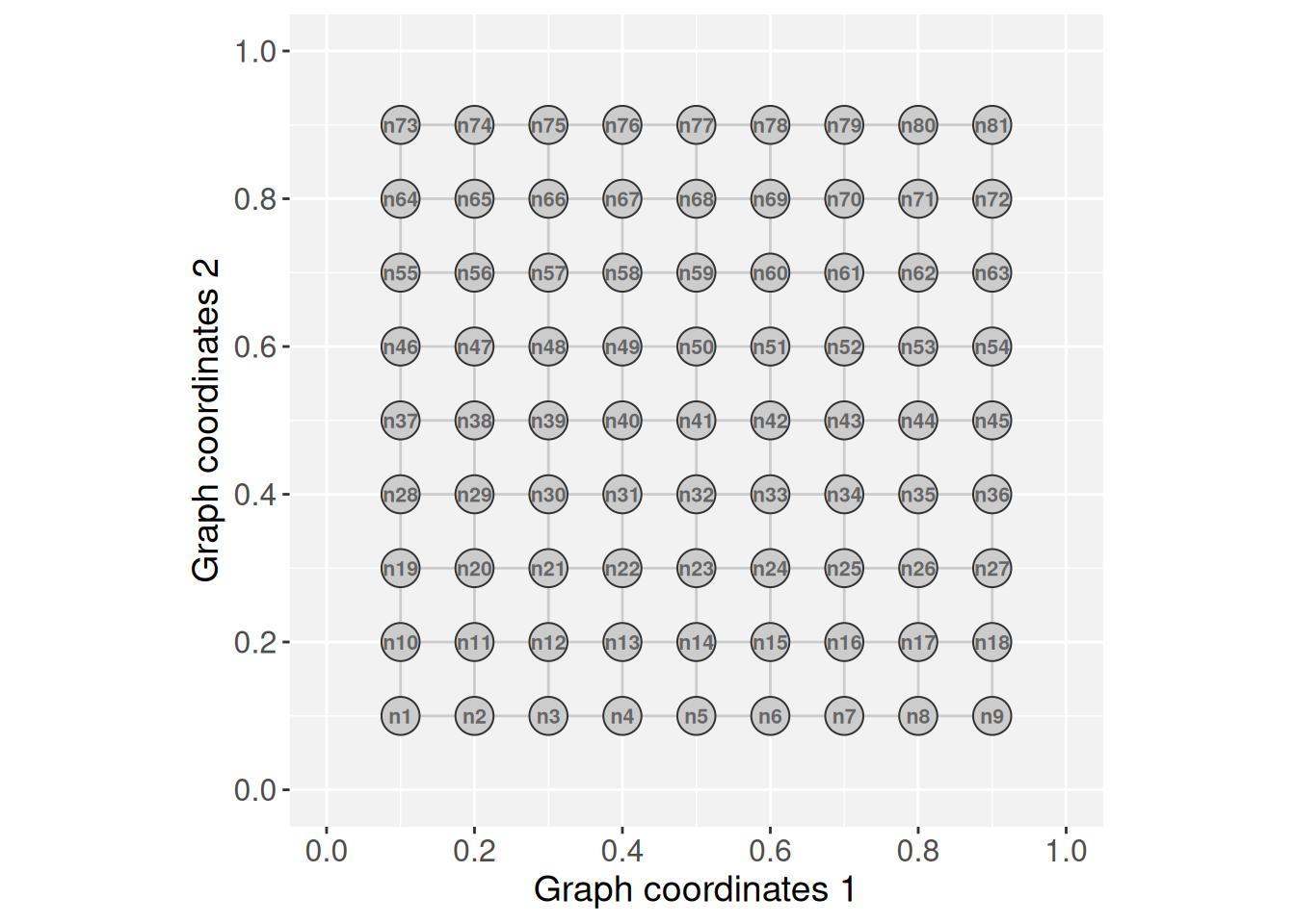
# Build a PathwaySpace object
ps <- buildPathwaySpace(gs)
Creating a decay function
In the context of PathwaySpace, a decay function describes
how a signal decreases as a function of distance, modeling the gradual
loss of intensity. These functions are used to attenuate signals over
graph-based domains, so contributions from distant vertices are weighted
less than those nearby. PathwaySpace provides three built-in
decay function constructors, weibullDecay(),
expDecay(), and linearDecay(), all sharing a
consistent argument structure for practical use and comparison:
\[ \begin{gather} \small y = signal \times \text{decay}^{\left(\tfrac{x}{\text{pdist}}\right)^{\text{shape}}} && \scriptsize{(\text{Weibull})} \end{gather} \] \[ \begin{gather} \small y = signal \times \text{decay}^{\left(\tfrac{x}{\text{pdist}}\right)} && \scriptsize{(\text{Exponential})} \end{gather} \]
\[ \begin{gather} \small y = signal \times \Bigl(1 - (1 - \text{decay}) \times \tfrac{x}{\text{pdist}}\Bigr) \ & \scriptsize{(\text{Linear*})} \\ \end{gather} \\[10pt] \scriptstyle\text{*output clipped to prevent flipping sign} \]
where \(\textbf{signal}\) represents
the initial intensity, \(\textbf{decay}\) controls the rate of
attenuation, \(\textbf{x}\) is a vector
of normalized distances, \(\textbf{shape}\) adjusts the curvature of
the decay, \(\textbf{pdist}\) is a
normalization term, and \(\textbf{y}\)
is the resulting signal decay values. Next, the main arguments are
illustrated using the weibullDecay() constructor, which
returns a decay function with customized parameters.
weibullDecay(decay = 0.25, shape = 2, pdist = 0.75)## function (x, signal)
## {
## y <- signal * 0.25^((x/0.75)^2)
## return(y)
## }
## <environment: 0x55d3432cb568>
## attr(,"name")
## [1] "weibullDecay"… and to visualize how different parameters affect the signal
attenuation, rerun the weibullDecay() constructor with
plot = TRUE.
# Run Weibull constructor with decay = 0.5, shape = 1, and pdist = 0.25
p1 <- weibullDecay(decay = 0.4, shape = 1, pdist = 0.2, plot = TRUE)

# Run Weibull constructor with decay = 0.5, shape = 2, and pdist = 0.50
p2 <- weibullDecay(decay = 0.4, shape = 2, pdist = 0.4, plot = TRUE)

# Run Weibull constructor with decay = 0.25, shape = 3, and pdist = 0.75
p3 <- weibullDecay(decay = 0.2, shape = 4, pdist = 0.8, plot = TRUE)

p1 + p2 + p3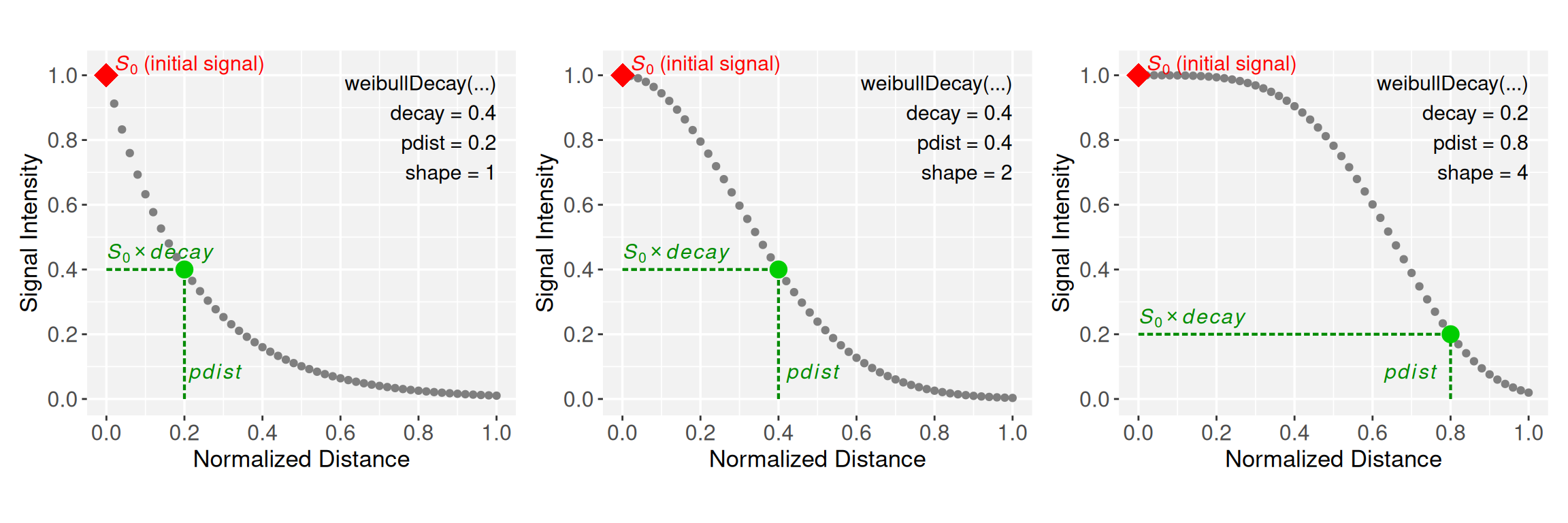
Note that the normalization term \(\textbf{pdist}\) anchors the decay to a reference distance where the initial signal \(S_0\) decreases to \(S_0 * \textbf{decay}\), controlling the extent over which the signal is projected along the x-axis. The \(\textbf{shape}\) parameter, on the other hand, controls the curvature of the decay function: When \(\textbf{shape} = 1\), the function follows an exponential decay; and for \(\textbf{shape} > 1\), the curve transitions from convex to concave, increasingly sigmoidal.
Next, we demonstrate the expDecay() and
linearDecay() constructors:
# Run the exp expDecay constructor with decay = 0.4 and pdist = 0.2
p1 <- expDecay(decay = 0.4, pdist = 0.2, plot = TRUE)

# Run the linearDecay constructor with decay = 0.5,and pdist = 0.25
p2 <- linearDecay(decay = 0.4, pdist = 0.3, plot = TRUE)

p1 + p2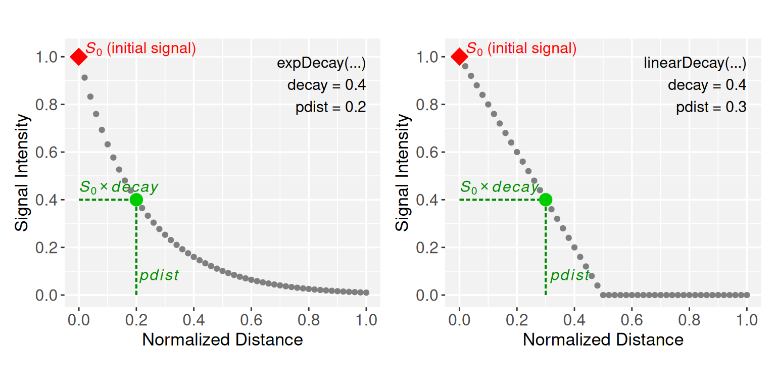
The exponential model follows an asymptotic decay, while the linear model decreases proportionally with distance and is clipped at zero to prevent flipping sign. Together, these decay models produce distinct geometric profiles when projecting signals onto the 2D coordinate space, ranging from cone-like projections in the linear model (see the conceptual representation in Figure 1A) to radially symmetric peaks in the exponential model, with the Weibull model transitioning between them to form dome-like surfaces depending on its \(\textbf{shape}\) parameter.
Assigning a decay model
Returning to our lattice example, next we assign a linear decay model
to the PathwaySpace object, setting \(\textbf{pdist}\) as the average
center-to-center distance between vertices. For more details, refer to
the documentation of the vertexDecay() accessor.
# Get distance to the nearest vertex
near_df <- getNearestNode(ps)
pdist <- mean(near_df$dist)
# 'pdist' set as the average center-to-center distance between vertices
pdist
## [1] 0.1# Setting a linear decay model for all vertices
vertexDecay(ps) <- linearDecay(pdist = pdist)Running PathwaySpace
Now we project a random binary signal using the
circularProjection() function.
# Add a random binary signal
set.seed(10)
vertexSignal(ps) <- sample(c(0,1), gs_vcount(ps), replace = TRUE)
# Running and plotting projections
ps <- circularProjection(ps, k = 1)
plotPathwaySpace(ps, marks = "n34")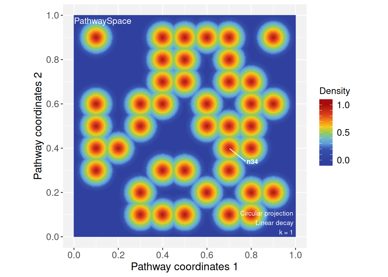
By assigning a new decay model to specific vertices, we can explore
how signals propagate across the network under different rules. To
illustrate, we assign a Weibull decay function to vertex
n34.
# Changing decay model of vertex 'n34'
vertexDecay(ps)[["n34"]] <- weibullDecay(shape = 2, pdist = pdist*10)
# Running and plotting projections
ps <- circularProjection(ps, k = 1)
plotPathwaySpace(ps, marks = "n34")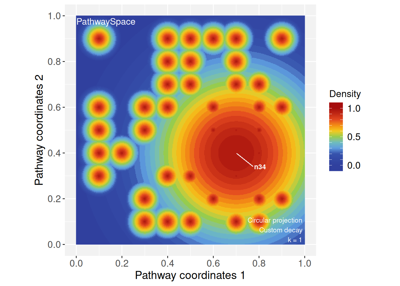
Session information
## R version 4.5.2 (2025-10-31)
## Platform: x86_64-pc-linux-gnu
## Running under: Ubuntu 24.04.4 LTS
##
## Matrix products: default
## BLAS:   /usr/lib/x86_64-linux-gnu/openblas-pthread/libblas.so.3
## LAPACK: /usr/lib/x86_64-linux-gnu/openblas-pthread/libopenblasp-r0.3.26.so;  LAPACK version 3.12.0
##
## locale:
##  [1] LC_CTYPE=en_US.UTF-8       LC_NUMERIC=C
##  [3] LC_TIME=en_US.UTF-8        LC_COLLATE=en_US.UTF-8
##  [5] LC_MONETARY=en_US.UTF-8    LC_MESSAGES=en_US.UTF-8
##  [7] LC_PAPER=en_US.UTF-8       LC_NAME=C
##  [9] LC_ADDRESS=C               LC_TELEPHONE=C
## [11] LC_MEASUREMENT=en_US.UTF-8 LC_IDENTIFICATION=C
##
## time zone: America/Sao_Paulo
## tzcode source: system (glibc)
##
## attached base packages:
## [1] stats     graphics  grDevices utils     datasets  methods   base
##
## other attached packages:
## [1] patchwork_1.3.2    igraph_2.2.0       SpotSpace_0.0.6    PathwaySpace_1.1.2
## [5] RGraphSpace_1.1.2  ggplot2_4.0.0.9000 remotes_2.5.0      bs4cards_0.1.1
##
## loaded via a namespace (and not attached):
##   [1] RColorBrewer_1.1-3     rstudioapi_0.17.1      jsonlite_2.0.0
##   [4] shape_1.4.6.1          magrittr_2.0.4         spatstat.utils_3.2-0
##   [7] ggbeeswarm_0.7.2       farver_2.1.2           rmarkdown_2.30
##  [10] GlobalOptions_0.1.2    fs_1.6.6               vctrs_0.6.5
##  [13] ROCR_1.0-11            spatstat.explore_3.5-3 htmltools_0.5.8.1
##  [16] sass_0.4.10            sctransform_0.4.2      parallelly_1.45.1
##  [19] KernSmooth_2.23-26     bslib_0.9.0            htmlwidgets_1.6.4
##  [22] ica_1.0-3              fontawesome_0.5.3      plyr_1.8.9
##  [25] plotly_4.11.0          zoo_1.8-14             cachem_1.1.0
##  [28] mime_0.13              lifecycle_1.0.4        pkgconfig_2.0.3
##  [31] Matrix_1.7-4           R6_2.6.1               fastmap_1.2.0
##  [34] fitdistrplus_1.2-4     future_1.67.0          shiny_1.11.1
##  [37] digest_0.6.37          colorspace_2.1-1       Seurat_5.4.0.9009
##  [40] tensor_1.5.1           RSpectra_0.16-2        irlba_2.3.5.1
##  [43] progressr_0.17.0       spatstat.sparse_3.1-0  httr_1.4.7
##  [46] polyclip_1.10-7        abind_1.4-8            compiler_4.5.2
##  [49] withr_3.0.2            S7_0.2.0               fastDummies_1.7.5
##  [52] MASS_7.3-65            tools_4.5.2            vipor_0.4.7
##  [55] lmtest_0.9-40          beeswarm_0.4.0         httpuv_1.6.16
##  [58] future.apply_1.20.0    goftest_1.2-3          glue_1.8.0
##  [61] nlme_3.1-168           promises_1.3.3         grid_4.5.2
##  [64] Rtsne_0.17             cluster_2.1.8.2        reshape2_1.4.4
##  [67] generics_0.1.4         gtable_0.3.6           spatstat.data_3.1-8
##  [70] tidyr_1.3.1            data.table_1.17.8      sp_2.2-0
##  [73] spatstat.geom_3.6-0    RcppAnnoy_0.0.22       ggrepel_0.9.6
##  [76] RANN_2.6.2             pillar_1.11.1          stringr_1.5.2
##  [79] spam_2.11-1            RcppHNSW_0.6.0         later_1.4.4
##  [82] circlize_0.4.16        splines_4.5.2          dplyr_1.1.4
##  [85] lattice_0.22-9         survival_3.8-6         deldir_2.0-4
##  [88] tidyselect_1.2.1       miniUI_0.1.2           pbapply_1.7-4
##  [91] knitr_1.50             gridExtra_2.3          scattermore_1.2
##  [94] xfun_0.54              matrixStats_1.5.0      stringi_1.8.7
##  [97] lazyeval_0.2.2         yaml_2.3.10            evaluate_1.0.5
## [100] codetools_0.2-20       tibble_3.3.0           cli_3.6.5
## [103] uwot_0.2.3             xtable_1.8-4           reticulate_1.44.1
## [106] jquerylib_0.1.4        dichromat_2.0-0.1      Rcpp_1.1.0
## [109] globals_0.18.0         spatstat.random_3.4-2  png_0.1-8
## [112] ggrastr_1.0.2          spatstat.univar_3.1-4  parallel_4.5.2
## [115] dotCall64_1.2          listenv_0.9.1          viridisLite_0.4.2
## [118] scales_1.4.0           ggridges_0.5.7         SeuratObject_5.3.0
## [121] purrr_1.1.0            rlang_1.1.6            cowplot_1.2.0